09- Logistic Regression Code Demo

Author

Dr. Cheng-Han Yu

1 R implementation

Code

library(ISLR2)

1.1 Binary (Binomial) Logistic Regression

Code

data("Default")
logit_fit <- glm(default ~ balance, data = Default, family = binomial)
coef(summary(logit_fit))

                 Estimate   Std. Error   z value      Pr(>|z|)
(Intercept) -10.651330614 0.3611573721 -29.49221 3.623124e-191
balance       0.005498917 0.0002203702  24.95309 1.976602e-137

Code

pi_hat <- predict(logit_fit, type = "response")
eta_hat <- predict(logit_fit, type = "link")  ## default gives us b0 + b1*x
predict(logit_fit, newdata = data.frame(balance = 2000), type = "response")

        1 
0.5857694

Code

pred_prob <- predict(logit_fit, type = "response")
table(pred_prob > 0.5, Default$default)

       
          No  Yes
  FALSE 9625  233
  TRUE    42  100

Code

library(ROCR)
# create an object of class prediction 
pred <- ROCR::prediction(predictions = pred_prob, labels = Default$default)

# calculates the ROC curve
roc <- ROCR::performance(prediction.obj = pred, measure = "tpr", x.measure = "fpr")
plot(roc, colorize = TRUE, lwd = 3)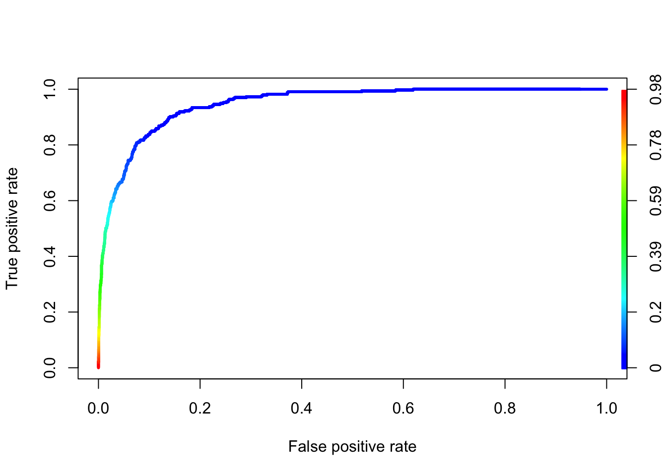

Code

auc <- ROCR::performance(prediction.obj = pred, measure = "auc")
auc@y.values

[[1]]
[1] 0.9479785

1.2 Multinomial Logistic Regression

Code

library(foreign)
multino_data <- foreign::read.dta("../data/hsbdemo.dta")

Code

multino_data$prog2 <- relevel(multino_data$prog, ref = "academic")
levels(multino_data$prog2)

[1] "academic" "general"  "vocation"

Code

levels(multino_data$ses)

[1] "low"    "middle" "high"

Code

library(nnet)
multino_fit <- nnet::multinom(prog2 ~ ses + write, data = multino_data, trace = FALSE)
summ <- summary(multino_fit)
summ$coefficients

         (Intercept)  sesmiddle    seshigh      write
general     2.852198 -0.5332810 -1.1628226 -0.0579287
vocation    5.218260  0.2913859 -0.9826649 -0.1136037

Code

head(fitted(multino_fit))

   academic   general  vocation
1 0.1482764 0.3382454 0.5134781
2 0.1202017 0.1806283 0.6991700
3 0.4186747 0.2368082 0.3445171
4 0.1726885 0.3508384 0.4764731
5 0.1001231 0.1689374 0.7309395
6 0.3533566 0.2377976 0.4088458

Code

dses <- data.frame(ses = c("low", "middle", "high"), 
                   write = mean(multino_data$write))
predict(multino_fit, newdata = dses, type = "probs")

   academic   general  vocation
1 0.4396845 0.3581917 0.2021238
2 0.4777488 0.2283353 0.2939159
3 0.7009007 0.1784939 0.1206054

We can also use glmnet package.

Code

library(fastDummies) # https://jacobkap.github.io/fastDummies/
library(glmnet)

Loading required package: Matrix

Loaded glmnet 4.1-8

Code

prog <- multino_data$prog2
dummy_dat <- dummy_cols(multino_data, select_columns = c("ses"))
x <- dummy_dat |> dplyr::select(ses_middle, ses_high, write)
fit <- glmnet(x = x, y = prog, family = "multinomial", lambda = 0)
coef(fit)

$academic
4 x 1 sparse Matrix of class "dgCMatrix"
                    s0
           -2.69052260
ses_middle  .         
ses_high    0.98278066
write       0.05793834

$general
4 x 1 sparse Matrix of class "dgCMatrix"
                   s0
            0.1625919
ses_middle -0.5337675
ses_high   -0.1805596
write       .        

$vocation
4 x 1 sparse Matrix of class "dgCMatrix"
                    s0
            2.52793069
ses_middle  0.29119238
ses_high    .         
write      -0.05566551

Code

newx <- x[1:3, ]
newx[, 3] <- mean(multino_data$write)
predict(fit, as.matrix(newx), type="response")

, , s0

   academic   general  vocation
1 0.4396037 0.3582719 0.2021245
2 0.4777583 0.2283218 0.2939199
3 0.7009084 0.1784762 0.1206154

Code

# model_mat <- model.matrix(prog2~ses+write, data=multino_data)

2 Python implementation

2.1 Binary (Binomial) Logistic Regression

Code

import numpy as np
import pandas as pd
from sklearn.metrics import confusion_matrix
import matplotlib.pyplot as plt

Code

# Load your dataset
Default = pd.read_csv("../data/Default.csv")

Code

Default['default'] = Default['default'].map({'Yes': 1, 'No': 0})
from statsmodels.formula.api import logit
logit_fit = logit(formula='default ~ balance', data=Default).fit()

Optimization terminated successfully.
         Current function value: 0.079823
         Iterations 10

Code

logit_fit.summary2().tables[1]

               Coef.  Std.Err.          z          P>|z|     [0.025    0.975]
Intercept -10.651331  0.361169 -29.491287  3.723665e-191 -11.359208 -9.943453
balance     0.005499  0.000220  24.952404  2.010855e-137   0.005067  0.005931

Code

pi_hat = logit_fit.predict(Default[['balance']])  # Type = "response" in R
eta_hat = logit_fit.predict(Default[['balance']], which="linear")  # Type = "link" in R
new_data = pd.DataFrame({'balance': [2000]})
logit_fit.predict(new_data)

0    0.585769
dtype: float64

Code

from sklearn.metrics import confusion_matrix
pred_prob = logit_fit.predict(Default[['balance']])  # Type = "response" in R
# Create predictions based on a 0.5 threshold
pred_class = (pred_prob > 0.5).astype(int)  # Convert to binary class (0 or 1)
## C00: true negatives; C10: false negatives; C01: false postives; C11: true positives
confusion_matrix(y_true=Default['default'], y_pred=pred_class)

array([[9625,   42],
       [ 233,  100]])

Code

from sklearn.metrics import roc_curve, roc_auc_score

# Calculate the ROC curve
fpr, tpr, thresholds = roc_curve(Default['default'], pred_prob)

# Calculate the AUC (Area Under the Curve)
auc = roc_auc_score(Default['default'], pred_prob)
auc

0.9479784946837808

Code

plt.figure()
plt.plot(fpr, tpr, color='blue')
plt.plot([0, 1], [0, 1], color='gray', linestyle='--')  # Diagonal line
plt.xlabel('False Positive Rate (FPR)')
plt.ylabel('True Positive Rate (TPR)')
plt.show()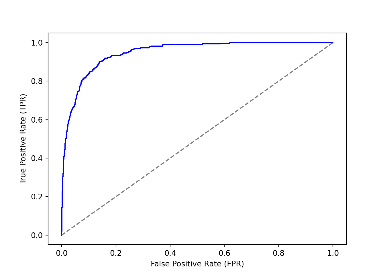

2.2 Multinomial Logistic Regression

Code

multino_data = pd.read_stata("../data/hsbdemo.dta")

Code

multino_data['prog2'] = multino_data['prog'].cat.reorder_categories(
    ['academic'] + [cat for cat in multino_data['prog'].cat.categories if cat != 'academic'],
    ordered=True
)
multino_data['prog2'].unique()

['vocation', 'general', 'academic']
Categories (3, object): ['academic' < 'general' < 'vocation']

Code

multino_data['ses'].unique()

['low', 'middle', 'high']
Categories (3, object): ['low' < 'middle' < 'high']

Code

multino_data['prog_int'] = multino_data['prog2'].map({
    'academic': 0,
    'general': 1,
    'vocation': 2
})
multino_data['prog_int'] = multino_data['prog_int'].cat.codes

Code

from statsmodels.formula.api import mnlogit
multino_fit = mnlogit("prog_int ~ ses + write", data=multino_data).fit()

Optimization terminated successfully.
         Current function value: 0.899909
         Iterations 6

Code

multino_fit.params

                      0         1
Intercept      2.852186  5.218200
ses[T.middle] -0.533291  0.291393
ses[T.high]   -1.162832 -0.982670
write         -0.057928 -0.113603

Code

fitted_df = pd.DataFrame(multino_fit.predict(), 
                         columns=['academic', 'general', 'vocation'])
fitted_df.head()

   academic   general  vocation
0  0.148278  0.338249  0.513473
1  0.120203  0.180629  0.699168
2  0.418679  0.236808  0.344513
3  0.172690  0.350841  0.476468
4  0.100125  0.168938  0.730937

Code

dses = pd.DataFrame({
    'ses': ['low', 'middle', 'high'],
    'write': [multino_data['write'].mean()] * 3
})
multino_fit.predict(dses)

          0         1         2
0  0.439684  0.358193  0.202123
1  0.477749  0.228334  0.293917
2  0.700902  0.178493  0.120605

We can also use sklearn package.

Code

from sklearn.linear_model import LogisticRegression
from sklearn.preprocessing import OneHotEncoder
from sklearn.compose import ColumnTransformer
from sklearn.pipeline import Pipeline

# Separate features (X) and target (y)
X = multino_data[['ses', 'write']]  # Independent variables
y = multino_data['prog_int']          # Dependent variable (categorical target)

preprocessor = ColumnTransformer(
    transformers=[
        ('cat', OneHotEncoder(drop='first'), ['ses']),  # One-hot encode 'ses'
        ('num', 'passthrough', ['write'])              # Leave 'write' as is
    ]
)
# Create a multinomial logistic regression model
model = Pipeline([
    ('preprocessor', preprocessor),  # Preprocessing step
    ('classifier', LogisticRegression(multi_class='multinomial', penalty=None,
                                      solver='lbfgs', max_iter=500))
])

model.fit(X, y)

Pipeline(steps=[('preprocessor',
                 ColumnTransformer(transformers=[('cat',
                                                  OneHotEncoder(drop='first'),
                                                  ['ses']),
                                                 ('num', 'passthrough',
                                                  ['write'])])),
                ('classifier',
                 LogisticRegression(max_iter=500, multi_class='multinomial',
                                    penalty=None))])

In a Jupyter environment, please rerun this cell to show the HTML representation or trust the notebook.
On GitHub, the HTML representation is unable to render, please try loading this page with nbviewer.org.

Code

model.named_steps.classifier.coef_

array([[-0.71516627, -0.63453974,  0.05717724],
       [ 0.4476491 , -0.0049987 , -0.00075151],
       [ 0.26751717,  0.63953844, -0.05642573]])

Code

model.named_steps.classifier.intercept_

array([-1.97496981, -0.28559419,  2.260564  ])

Code

dses = pd.DataFrame({
    'ses': ['low', 'middle', 'high'],
    'write': [multino_data['write'].mean()] * 3
})

pd.DataFrame(model.predict_proba(dses),
             columns=model.named_steps.classifier.classes_)

          0         1         2
0  0.439686  0.358190  0.202124
1  0.477748  0.228334  0.293917
2  0.700903  0.178494  0.120603