14 - Tree Methods Code Demo

Author

Dr. Cheng-Han Yu

1 R implementation

Code

# generate some data 
set.seed(2025)
n <- 1000
x1 <- runif(n, -1, 1)
x2 <- runif(n, -1, 1)
y <- rbinom(n, size = 1, prob = ifelse((x1 + x2 > -0.5) & (x1 + x2 < 0.5) , 0.8, 0.2))
xgrid <- expand.grid(x1 = seq(-1, 1, 0.01), x2 = seq(-1, 1, 0.01))

1.1 CART

1.1.1 rpart::rpart()

Code

library(rpart)
rpart_fit <- rpart(as.factor(y) ~ x1 + x2, data = data.frame(x1, x2, y))
pred <- matrix(predict(rpart_fit, xgrid, type = "class") == 1, 201, 201)
contour(seq(-1, 1, 0.01), seq(-1, 1, 0.01), pred, levels = 0.5, labels = "",
        lwd = 3)
points(xgrid, pch = ".", cex = 0.2, col = ifelse(pred, "lightblue", "pink"))
points(x1, x2, col = ifelse(y == 1, 4, 2), pch = 19, yaxt = "n", xaxt = "n")
box()
title(main = list("CART"))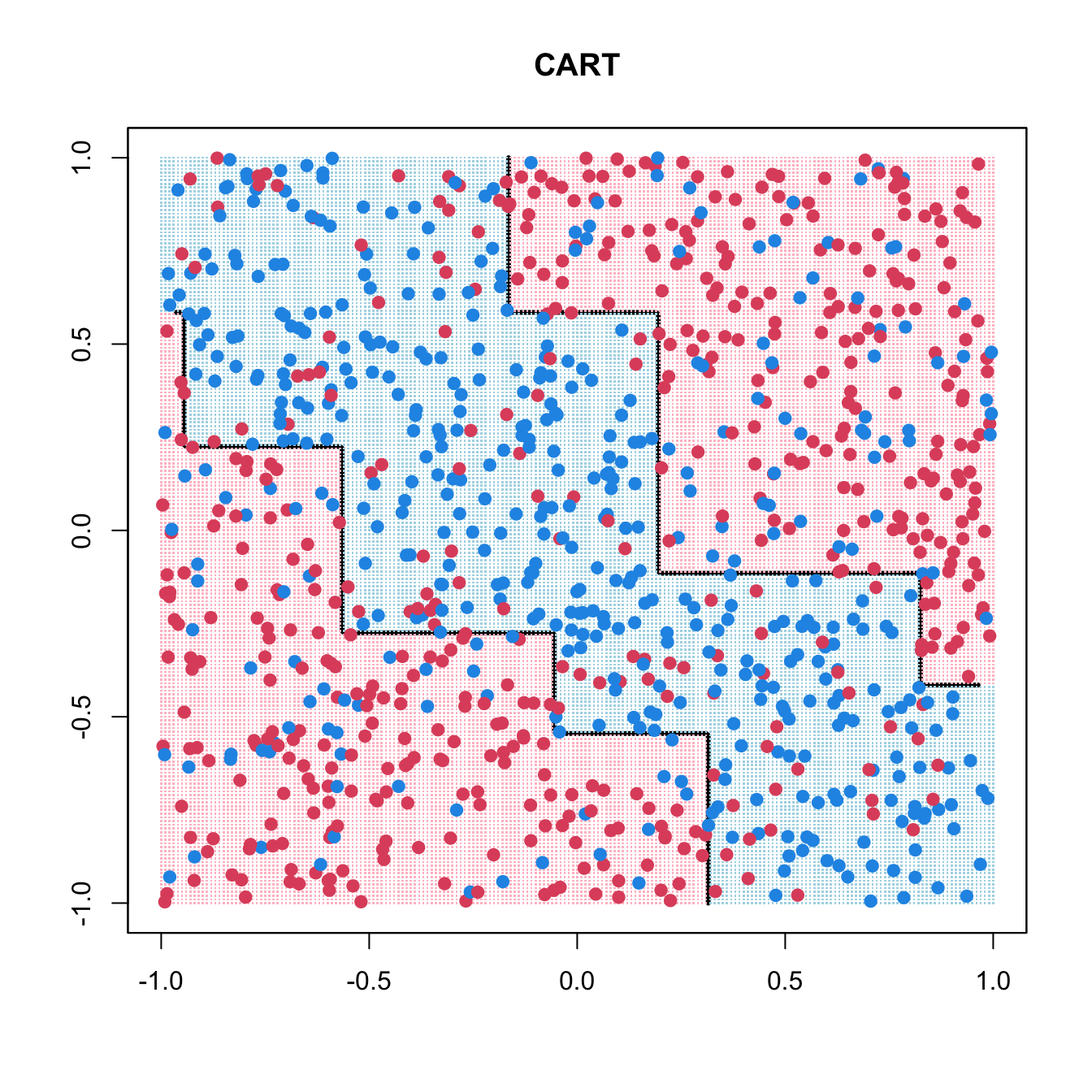

Code

par(mar = c(0.5, 0, 0.5, 0))
plot(rpart_fit)
text(rpart_fit, cex = 0.8)

rpart() uses the 10-fold CV (xval in rpart.control())
cp is the complexity parameter

Code

rpart.control(minsplit = 20, minbucket = round(minsplit/3), cp = 0.01, 
              maxcompete = 4, maxsurrogate = 5, usesurrogate = 2, xval = 10,
              surrogatestyle = 0, maxdepth = 30, ...)

Code

rpart_fit$cptable

          CP nsplit rel error    xerror       xstd
1 0.06485356      0 1.0000000 1.0000000 0.03304618
2 0.05857741      3 0.7845188 0.9058577 0.03277990
3 0.05439331      4 0.7259414 0.8284519 0.03235476
4 0.03242678      5 0.6715481 0.7050209 0.03127115
5 0.02719665      9 0.5418410 0.6401674 0.03048685
6 0.01464435     10 0.5146444 0.6087866 0.03004981
7 0.01359833     11 0.5000000 0.5732218 0.02950636
8 0.01000000     13 0.4728033 0.5732218 0.02950636

Code

plotcp(rpart_fit)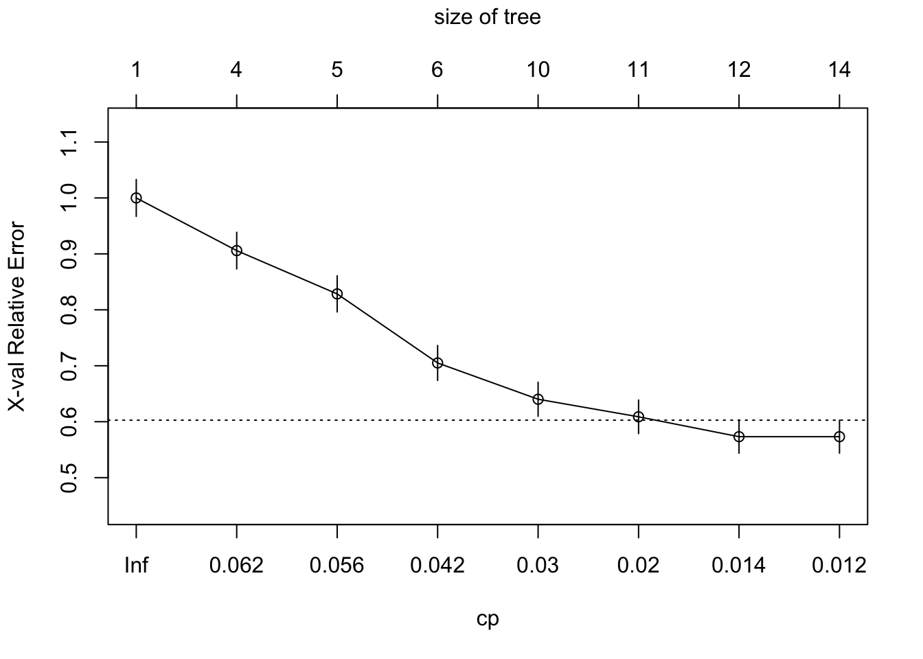

Code

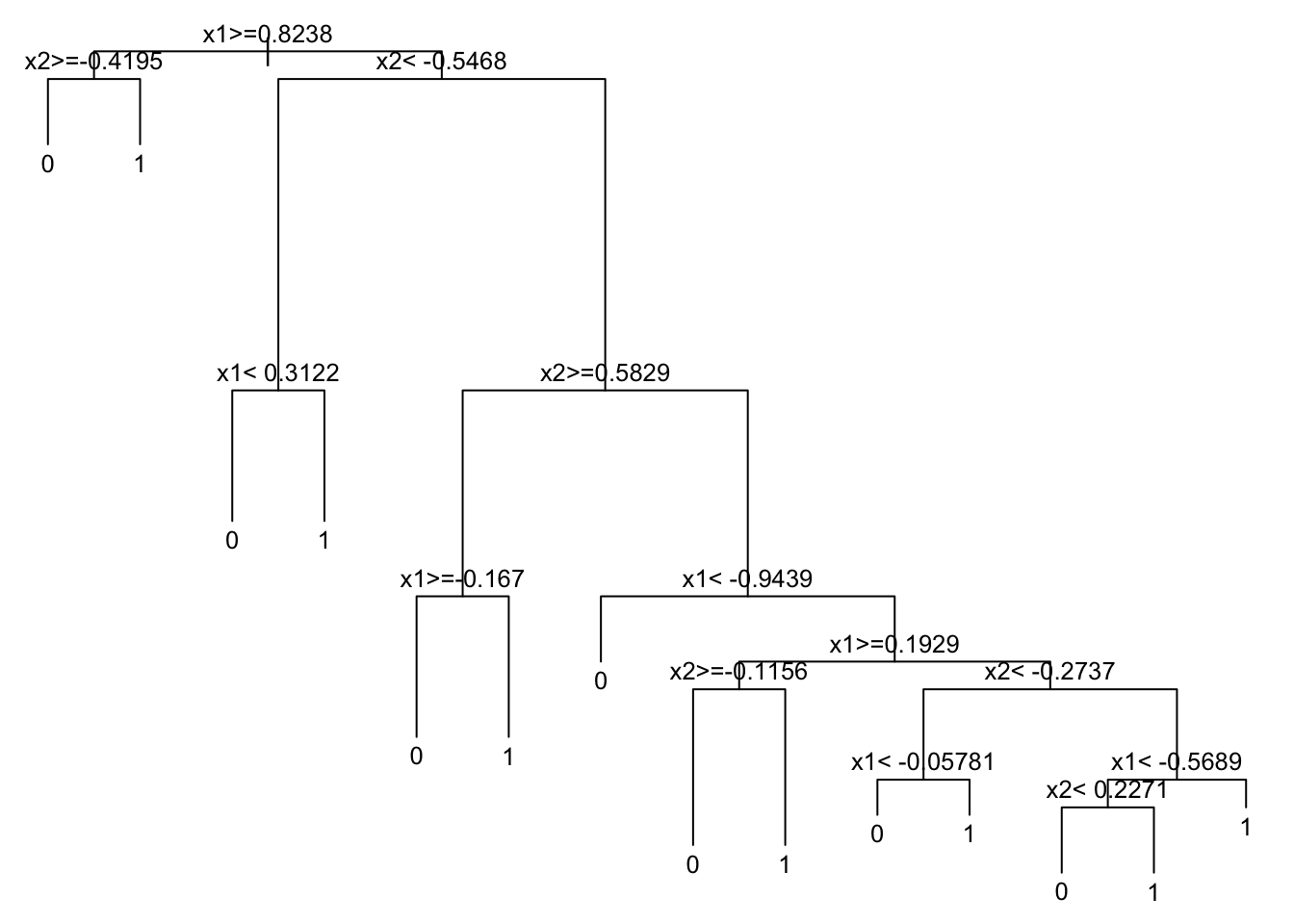
prunedtree <- prune(rpart_fit, cp = 0.012)
prunedtree

n= 1000 

node), split, n, loss, yval, (yprob)
      * denotes terminal node

  1) root 1000 478 0 (0.5220000 0.4780000)  
    2) x1>=0.8238083 93  26 0 (0.7204301 0.2795699)  
      4) x2>=-0.4195459 74  10 0 (0.8648649 0.1351351) *
      5) x2< -0.4195459 19   3 1 (0.1578947 0.8421053) *
    3) x1< 0.8238083 907 452 0 (0.5016538 0.4983462)  
      6) x2< -0.546795 203  69 0 (0.6600985 0.3399015)  
       12) x1< 0.3121958 145  27 0 (0.8137931 0.1862069) *
       13) x1>=0.3121958 58  16 1 (0.2758621 0.7241379) *
      7) x2>=-0.546795 704 321 1 (0.4559659 0.5440341)  
       14) x2>=0.5828916 189  74 0 (0.6084656 0.3915344)  
         28) x1>=-0.1670433 115  23 0 (0.8000000 0.2000000) *
         29) x1< -0.1670433 74  23 1 (0.3108108 0.6891892) *
       15) x2< 0.5828916 515 206 1 (0.4000000 0.6000000)  
         30) x1< -0.9438582 17   2 0 (0.8823529 0.1176471) *
         31) x1>=-0.9438582 498 191 1 (0.3835341 0.6164659)  
           62) x1>=0.192903 169  79 1 (0.4674556 0.5325444)  
            124) x2>=-0.1156255 97  33 0 (0.6597938 0.3402062) *
            125) x2< -0.1156255 72  15 1 (0.2083333 0.7916667) *
           63) x1< 0.192903 329 112 1 (0.3404255 0.6595745)  
            126) x2< -0.2736896 80  31 0 (0.6125000 0.3875000)  
              252) x1< -0.05781444 57  16 0 (0.7192982 0.2807018) *
              253) x1>=-0.05781444 23   8 1 (0.3478261 0.6521739) *
            127) x2>=-0.2736896 249  63 1 (0.2530120 0.7469880)  
              254) x1< -0.568942 82  34 1 (0.4146341 0.5853659)  
                508) x2< 0.2270988 39  13 0 (0.6666667 0.3333333) *
                509) x2>=0.2270988 43   8 1 (0.1860465 0.8139535) *
              255) x1>=-0.568942 167  29 1 (0.1736527 0.8263473) *

Code

rpart.plot::rpart.plot(prunedtree)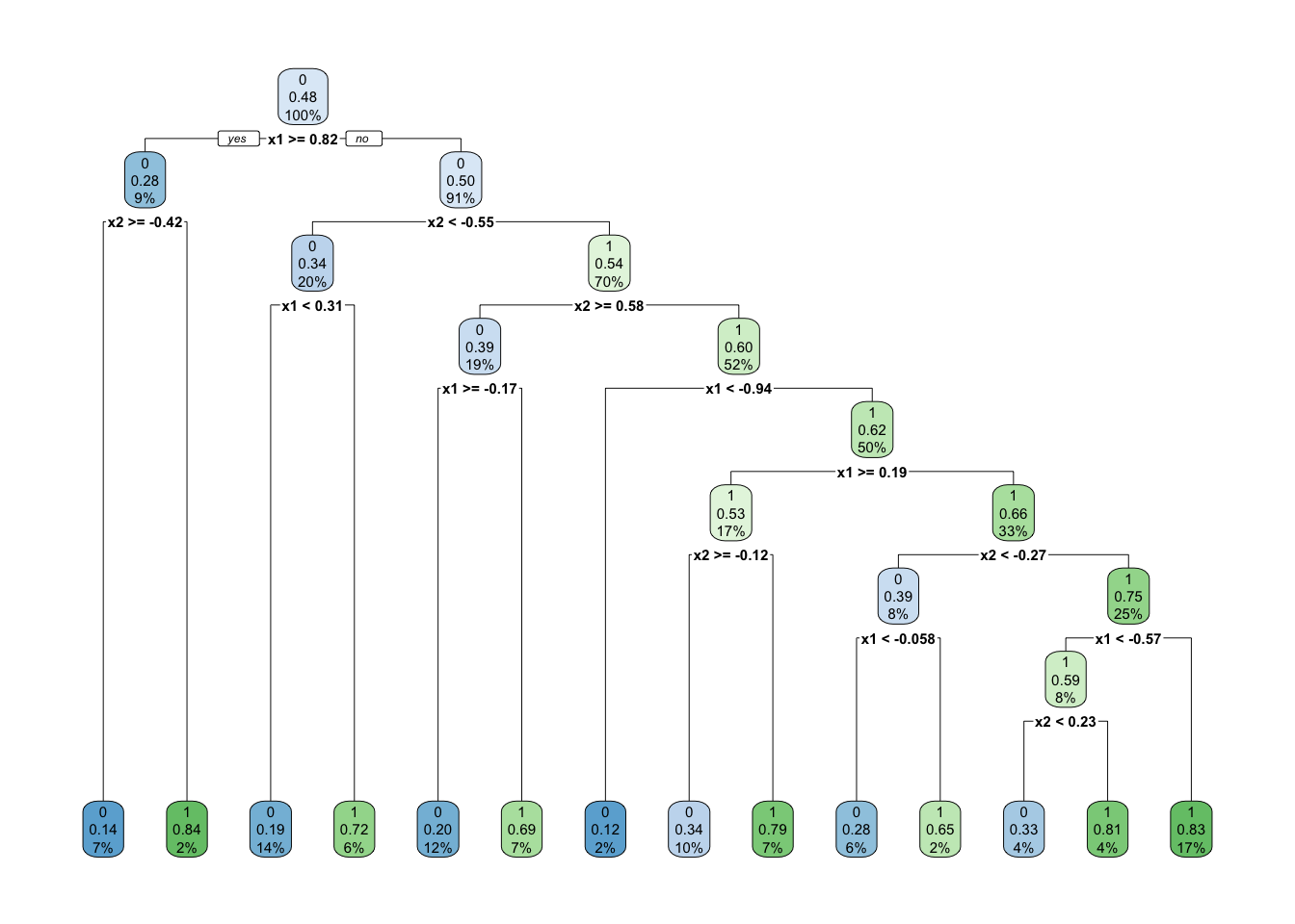

1.1.2 tree::tree()

Read ISLR Sec 8.3 for tree() demo.

1.2 Bagging

Code

library(ipred)
bag_fit <- bagging(as.factor(y) ~ x1 + x2, data = data.frame(x1, x2, y), 
                   nbagg = 200, ns = 400)
pred <- matrix(predict(prune(bag_fit), xgrid) == 1, 201, 201)
contour(seq(-1, 1, 0.01), seq(-1, 1, 0.01), pred, levels = 0.5, labels = "", 
        lwd = 3)
points(xgrid, pch = ".", cex = 0.2, col = ifelse(pred, "lightblue", "pink"))
points(x1, x2, col = ifelse(y == 1, 4, 2), pch = 19, yaxt = "n", xaxt = "n")
box()
title(main = list("Bagging"))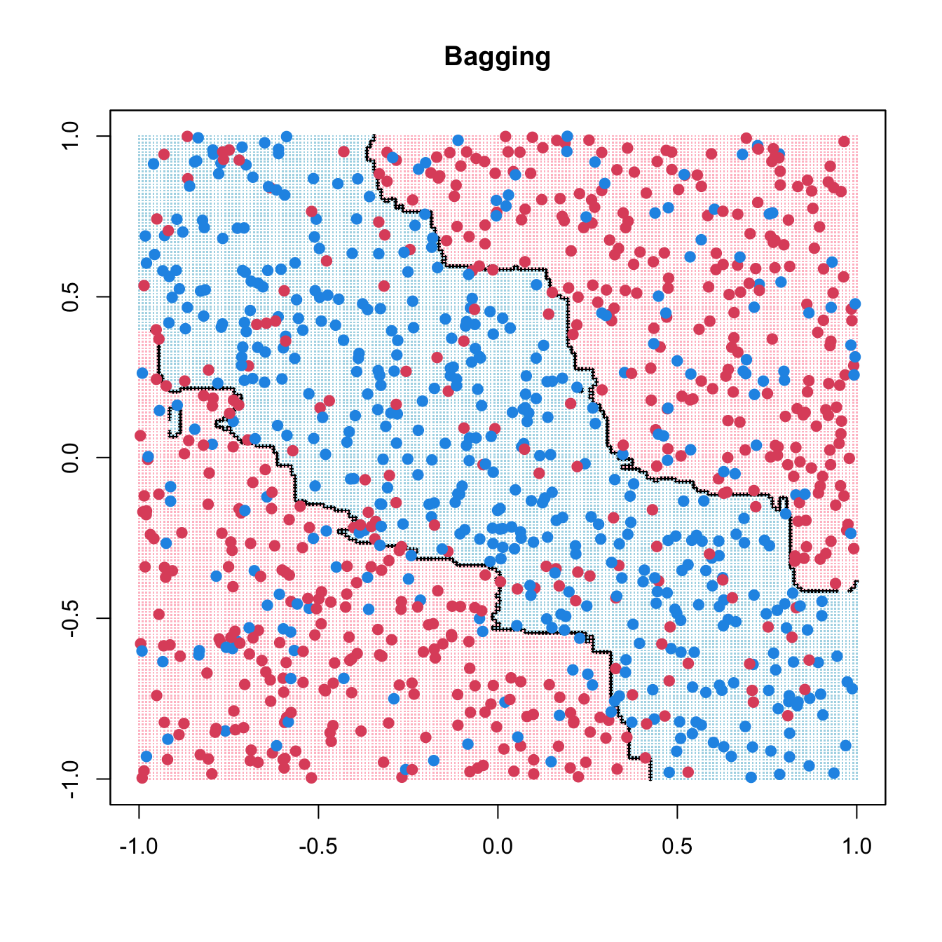

1.3 Random Forests

Code

library(randomForest)

randomForest 4.7-1.1

Type rfNews() to see new features/changes/bug fixes.

Code

rf_fit <- randomForest(cbind(x1, x2), as.factor(y), ntree = 200, mtry = 1, 
                      nodesize = 20, sampsize = 400)
pred <- matrix(predict(rf_fit, xgrid) == 1, 201, 201)
contour(seq(-1, 1, 0.01), seq(-1, 1, 0.01), pred, levels = 0.5, labels = "",
        lwd = 3)
points(xgrid, pch = ".", cex = 0.2, col = ifelse(pred, "lightblue", "pink"))
points(x1, x2, col = ifelse(y == 1, 4, 2), pch = 19, yaxt="n", xaxt = "n")
box()
title(main = list("Random Forests", cex = 2))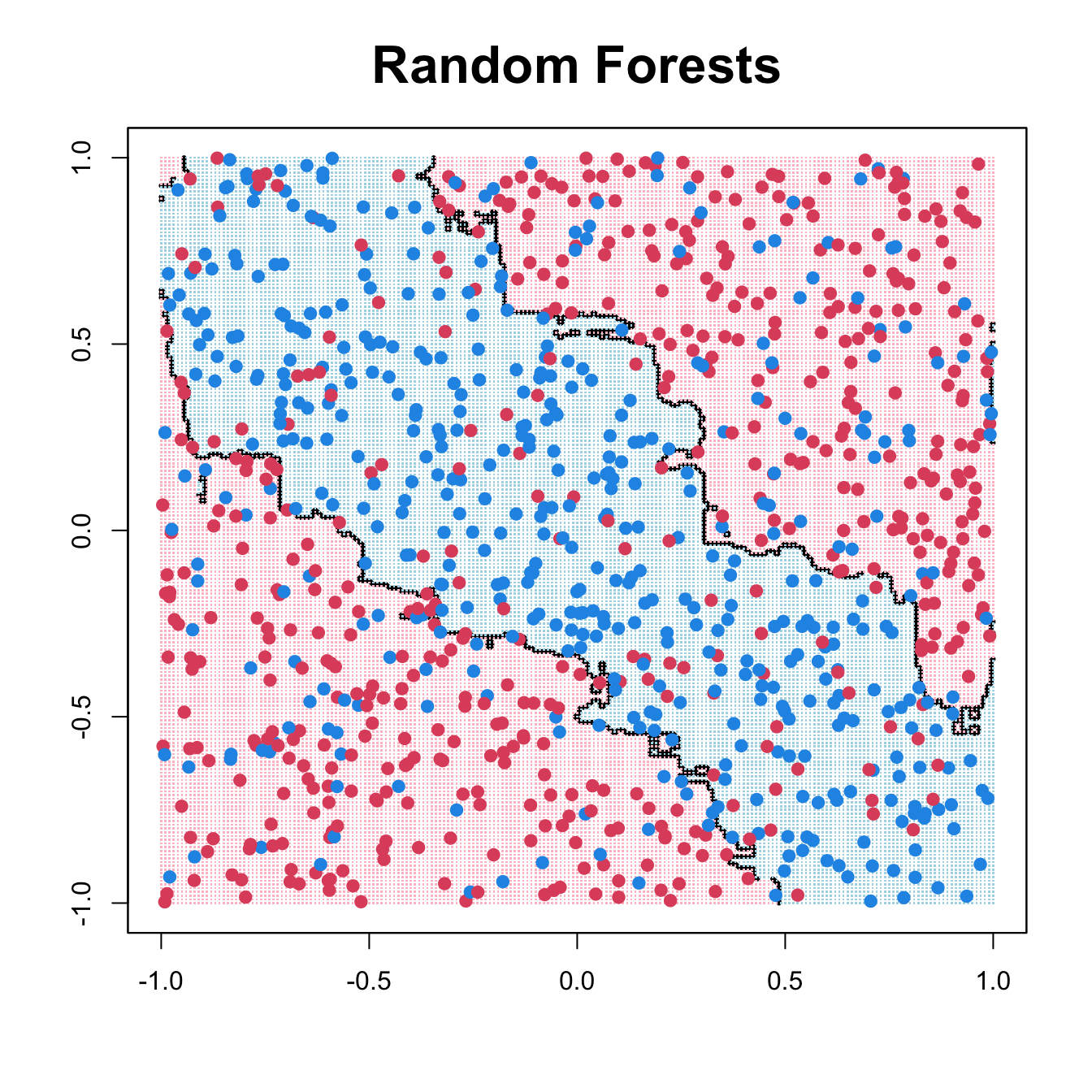

1.4 Boosting

Code

library(gbm)

Loaded gbm 2.2.2

This version of gbm is no longer under development. Consider transitioning to gbm3, https://github.com/gbm-developers/gbm3

Code

gbm_fit <- gbm(y ~ ., data = data.frame(x1, x2, y), distribution = "bernoulli", 
               n.trees = 10000, shrinkage = 0.01, bag.fraction = 0.6, 
               interaction.depth = 2, cv.folds = 10)
usetree <- gbm.perf(gbm_fit, method = "cv", plot.it = FALSE)
Fx <- predict(gbm_fit, xgrid, n.trees=usetree)
pred <- matrix(1 / (1 + exp(-2 * Fx)) > 0.5, 201, 201)
contour(seq(-1, 1, 0.01), seq(-1, 1, 0.01), pred, levels = 0.5, labels = "",
        lwd = 3)
points(xgrid, pch = ".", cex = 0.2, col = ifelse(pred, "lightblue", "pink"))
points(x1, x2, col = ifelse(y == 1, 4, 2), pch = 19, yaxt = "n", xaxt = "n")
box()
title(main = list("Boosting"))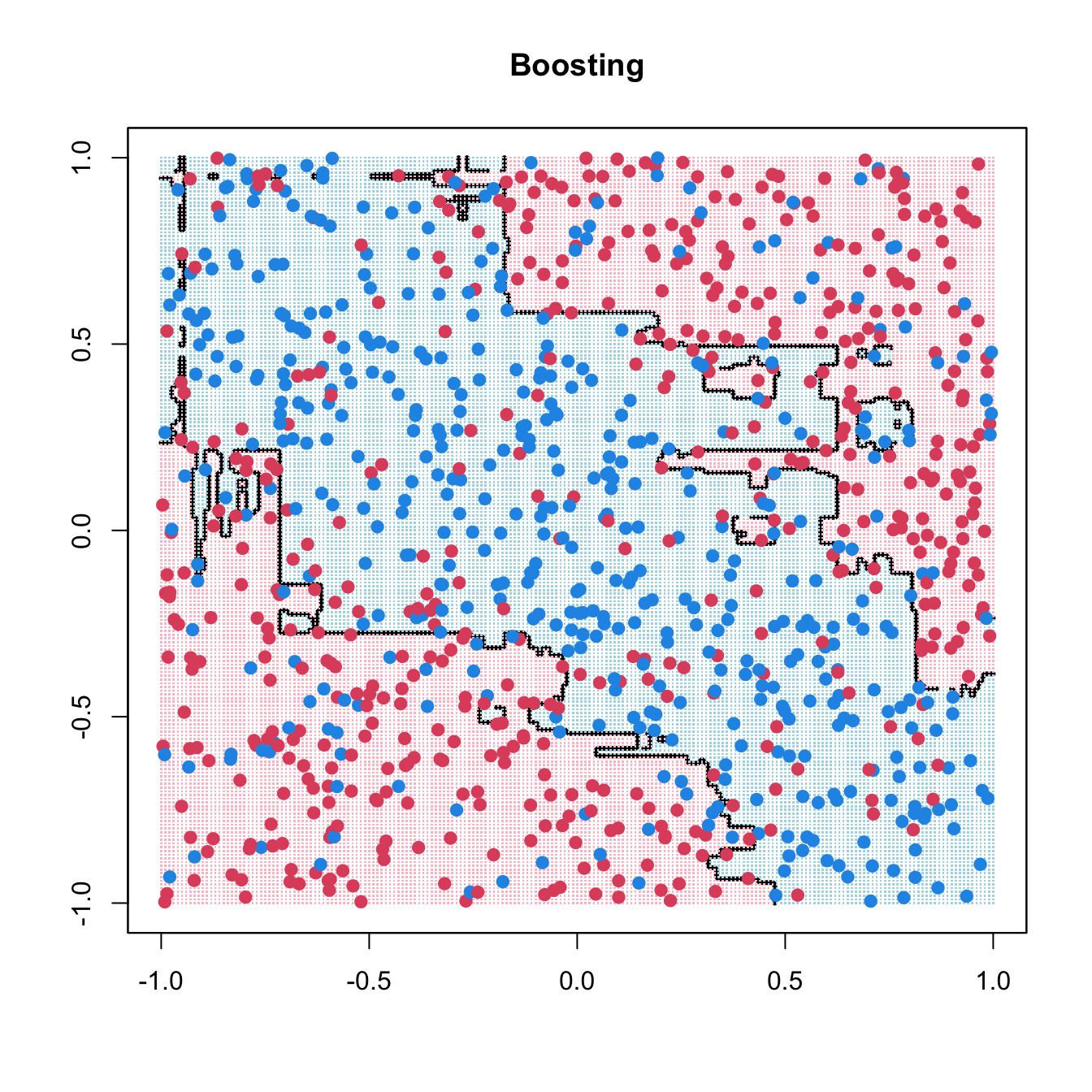

2 Python implementation

Code

import numpy as np
import matplotlib.pyplot as plt
from sklearn.tree import DecisionTreeClassifier
from sklearn.model_selection import GridSearchCV

Code

np.random.seed(2025)
n = 1000
x1 = np.random.uniform(-1, 1, n)
x2 = np.random.uniform(-1, 1, n)
y = np.random.binomial(1, p = np.where((x1 + x2 > -0.5) & (x1 + x2 < 0.5), 0.8, 0.2))
x1_grid, x2_grid = np.meshgrid(np.linspace(-1, 1, 201), np.linspace(-1, 1, 201))
xgrid = np.c_[x1_grid.ravel(), x2_grid.ravel()]

2.1 CART

Code

dt = DecisionTreeClassifier(random_state=2025)
param_grid = {
    "max_depth": [3, 5, 7, 10],  # Control tree depth
    "min_samples_split": [2, 5, 10],  # Minimum samples to split a node
    "min_samples_leaf": [1, 5, 10]  # Minimum samples in a leaf node
}
grid_search = GridSearchCV(dt, param_grid, cv=10, scoring="accuracy")
grid_search.fit(np.c_[x1, x2], y)

GridSearchCV(cv=10, estimator=DecisionTreeClassifier(random_state=2025),
             param_grid={'max_depth': [3, 5, 7, 10],
                         'min_samples_leaf': [1, 5, 10],
                         'min_samples_split': [2, 5, 10]},
             scoring='accuracy')

In a Jupyter environment, please rerun this cell to show the HTML representation or trust the notebook.
On GitHub, the HTML representation is unable to render, please try loading this page with nbviewer.org.

Code

best_dt = grid_search.best_estimator_
best_pred = best_dt.predict(xgrid).reshape(201, 201)

plt.figure()
plt.contourf(x1_grid, x2_grid, best_pred, cmap="coolwarm", alpha=0.3)
plt.scatter(x1, x2, c=y, cmap="bwr", s=15, alpha=0.7)
plt.xlabel("x1")
plt.ylabel("x2")
plt.title("CART")
plt.show()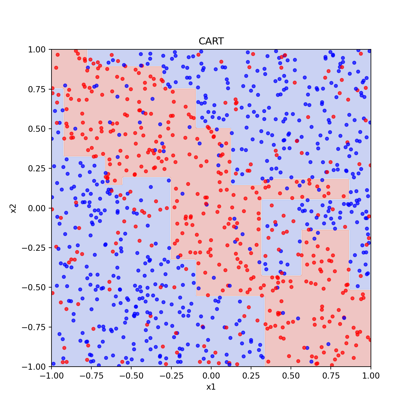

2.2 Bagging

Code

from sklearn.ensemble import BaggingClassifier

Code

bagging_clf = BaggingClassifier(
    estimator=DecisionTreeClassifier(),
    n_estimators=200,  # Same as nbagg = 200 in R
    max_samples=0.4,   # Equivalent to ns = 400 in R (approx)
    random_state=2025
)
bagging_clf.fit(np.c_[x1, x2], y)

BaggingClassifier(estimator=DecisionTreeClassifier(), max_samples=0.4,
                  n_estimators=200, random_state=2025)

Code

bagging_pred = bagging_clf.predict(xgrid).reshape(201, 201)
plt.figure()
plt.contourf(x1_grid, x2_grid, bagging_pred, cmap="coolwarm", alpha=0.3)
plt.scatter(x1, x2, c=y, cmap="bwr", s=15, alpha=0.7)
plt.xlabel("x1")
plt.ylabel("x2")
plt.title("Bagging")
plt.show()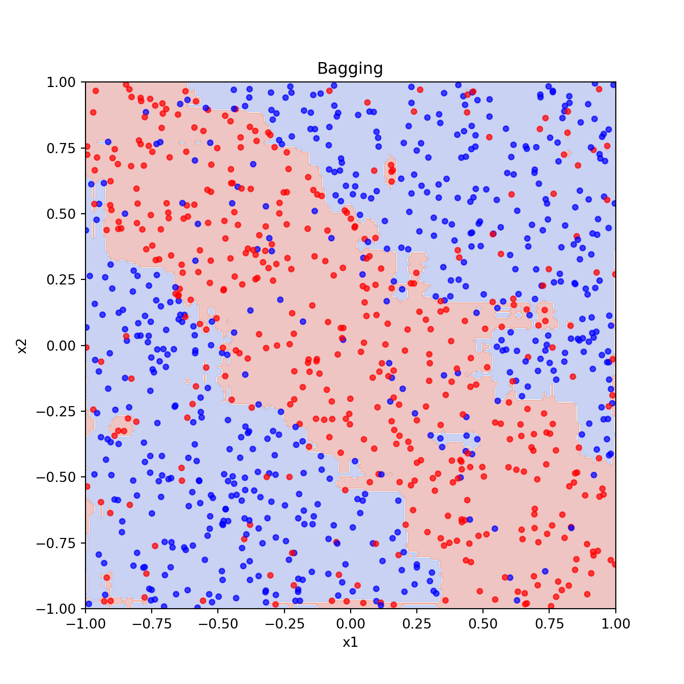

2.3 Random Forests

Code

from sklearn.ensemble import RandomForestClassifier

Code

rf_clf = RandomForestClassifier(
    n_estimators=200,  # Equivalent to ntree = 200 in R
    max_features=1,    # Equivalent to mtry = 1 in R
    min_samples_leaf=20,  # Equivalent to nodesize = 20 in R
    max_samples=400,  # Equivalent to sampsize = 400 in R
    random_state=2025
)
rf_clf.fit(np.c_[x1, x2], y)

RandomForestClassifier(max_features=1, max_samples=400, min_samples_leaf=20,
                       n_estimators=200, random_state=2025)

Code

rf_pred = rf_clf.predict(xgrid).reshape(201, 201)
plt.figure()
plt.contourf(x1_grid, x2_grid, rf_pred, cmap="coolwarm", alpha=0.3)
plt.scatter(x1, x2, c=y, cmap="bwr", s=15, alpha=0.7)
plt.xlabel("x1")
plt.ylabel("x2")
plt.title("Random Forests")
plt.show()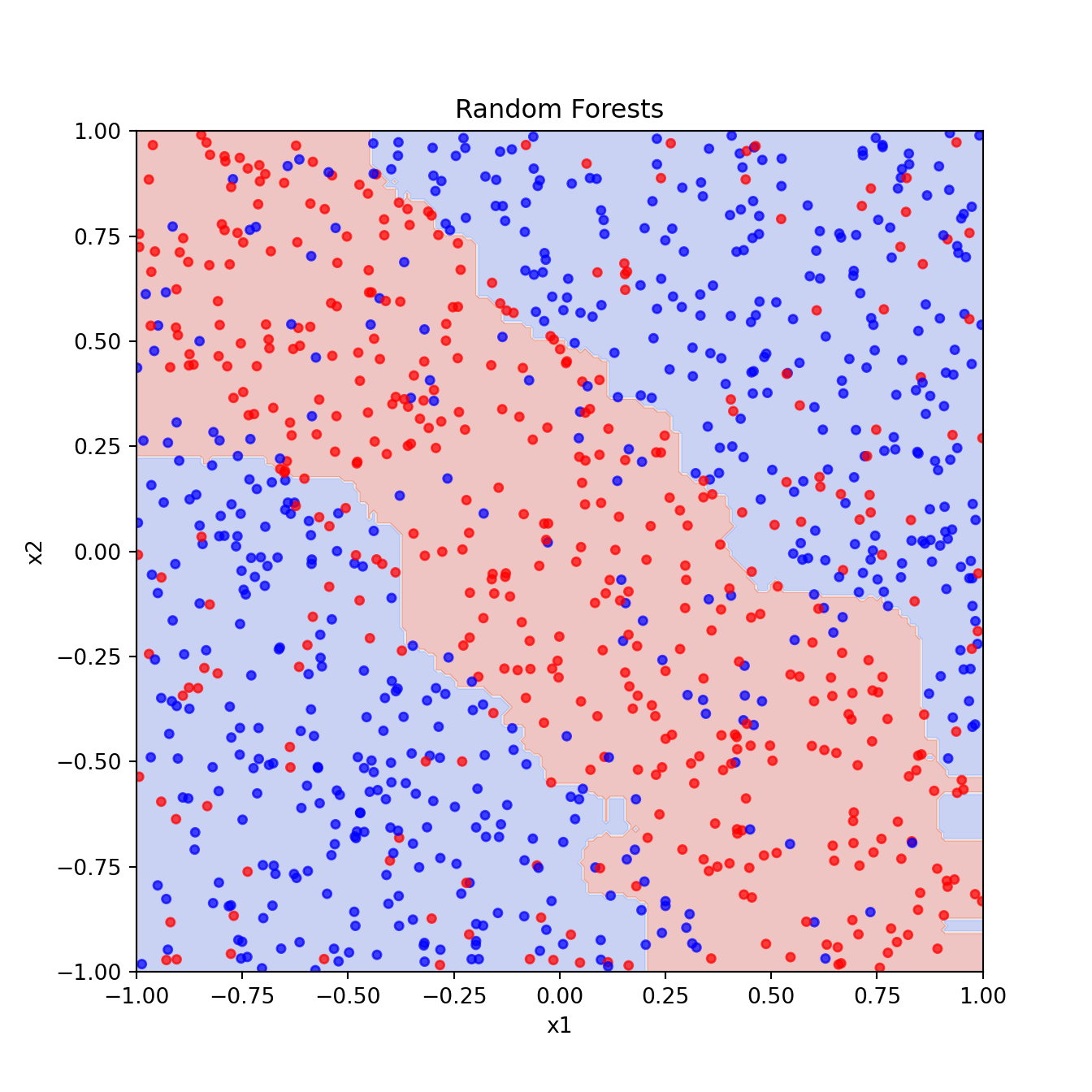

2.4 Boosting

Code

from sklearn.ensemble import GradientBoostingClassifier
from sklearn.model_selection import cross_val_score

Code

gbm_clf = GradientBoostingClassifier(
    n_estimators=10000,  # Equivalent to n.trees = 10000
    learning_rate=0.01,  # Equivalent to shrinkage = 0.01
    subsample=0.6,       # Equivalent to bag.fraction = 0.6
    max_depth=2,         # Equivalent to interaction.depth = 2
    random_state=2025
)
cv_scores = []
for n_trees in range(100, 2000, 100):  # Testing tree counts
    gbm_clf.set_params(n_estimators=n_trees)
    score = np.mean(cross_val_score(gbm_clf, np.c_[x1, x2], y, cv=10, scoring='accuracy'))
    cv_scores.append((n_trees, score))

GradientBoostingClassifier(learning_rate=0.01, max_depth=2, n_estimators=1900,
                           random_state=2025, subsample=0.6)

Code

best_n_trees = max(cv_scores, key=lambda x: x[1])[0]
gbm_clf.set_params(n_estimators=best_n_trees)

GradientBoostingClassifier(learning_rate=0.01, max_depth=2, n_estimators=500,
                           random_state=2025, subsample=0.6)

Code

gbm_clf.fit(np.c_[x1, x2], y)

GradientBoostingClassifier(learning_rate=0.01, max_depth=2, n_estimators=500,
                           random_state=2025, subsample=0.6)

Code

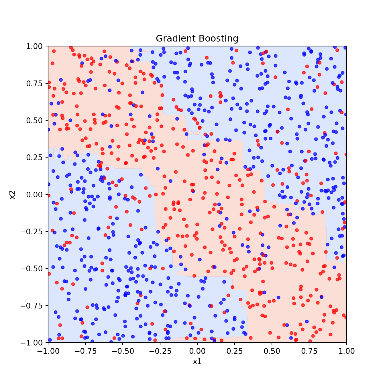
Fx = gbm_clf.decision_function(xgrid)  # Raw output before sigmoid transformation
pred = (1 / (1 + np.exp(-2 * Fx)) > 0.5).reshape(201, 201)
plt.figure()
plt.contourf(x1_grid, x2_grid, pred, cmap="coolwarm", alpha=0.3)
plt.scatter(x1, x2, c=y, cmap="bwr", s=15, alpha=0.7)
plt.xlabel("x1")
plt.ylabel("x2")
plt.title("Gradient Boosting")
plt.show()