Homework 1 - Bias-Variance Tradeoff and Linear Regression

Important

Due Friday, Feb 14, 11:59 PM

• Please submit your work in one PDF file to D2L > Assessments > Dropbox. Multiple files or a file that is not in pdf format are not allowed.

• Any relevant code should be attached.

• Problems started with (MSSC Phd) are required for CMPS PhD students, and optional for other students for extra credits.

• Readings: ISL Chapter 2 and 3.

Homework Problems

1. ISL Sec. 2.4: 1

2. ISL Sec. 2.4: 3

3. ISL Sec. 2.4: 5

4. ISL Sec. 3.7: 4

5. ISL Sec. 3.7: 6

6. ISL Sec. 3.7: 14

7. Simulation of simple linear regression. Consider the model \(y_i = \beta_0 + \beta_1x_i + \epsilon_i, ~~ \epsilon_i \stackrel{iid} \sim N(0, \sigma^2), ~~ i = 1, \dots, n,\) or equivalently, \(p(y_i \mid x, \beta_0, \beta_1) = N\left(\beta_0 + \beta_1x_i, \sigma^2 \right).\) Set \(\beta_0 = 2, \beta_1 = -1.5, \sigma = 1, n = 100, x_i = i.\) Generate 1000 simulated data sets and fit the model to each data set. The sampling distribution of the least-squares estimator \(b_1\) is \[b_1 \sim N\left(\beta_1, \frac{\sigma^2}{\sum_{i=1}^n (x_i - \bar{x})^2}\right).\]

   1. Find the average of the 1000 estimates \(b_1\). Is it close to its true expected value?

   2. Find the variance of 1000 estimates \(b_1\). Is it close to its true value?

   3. Draw the histogram of \(b_1\). Comment on your graph.

   4. Obtain 1000 95% confidence interval for \(\beta_1\). What is your pertentage of coverage for \(\beta_1\)? Comment your result.

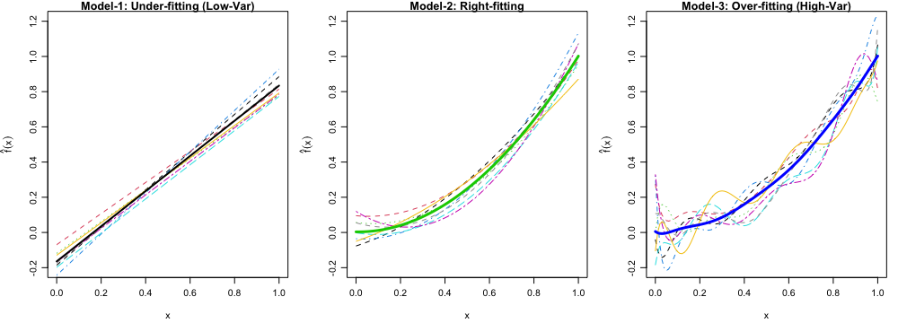
8. Simulation of bias-variance tradeoff. Let \(f(x) = x ^ 2\) be the true regression function. Simulate the data using \(y_i = f(x_i) + \epsilon_i, i = 1, \dots, 100\), where \(x_i = 0.01i\) and \(\epsilon_i \stackrel{iid} \sim N(0, 0.3^2).\)

   1. Generate 250 training data sets.
   2. For each data set, fit the following three models:
   • Model 1: \(y = \beta_0+\beta_1x+\epsilon\)
   • Model 2: \(y = \beta_0+\beta_1x+ \beta_2x^2 + \epsilon\)
   • Model 3: \(y = \beta_0+\beta_1x+ \beta_2x^2 + \cdots + \beta_9x^9 + \epsilon\)
   3. Calculate empirical MSE of \(\hat{f}\), bias of \(\hat{f}\) and variance of \(\hat{f}\). Then show that \[\text{MSE}_{\hat{f}} \approx \text{Bias}^2(\hat{f}) + \mathrm{Var}(\hat{f}).\] Specifically, for each value of \(x_i\), \(i = 1, \dots, 100\),

   \[\text{MSE}_{\hat{f}} = \frac{1}{250}\sum_{k=1}^{250} \left(\hat{f}_k(x_i) - f(x_i) \right) ^2,\] \[\text{Bias}(\hat{f}) = \overline{\hat{f}}(x_i) - f(x_i),\] where \(\overline{\hat{f}}(x_i) = \frac{1}{250}\sum_{k = 1}^{250}\hat{f}_k(x_i)\) is the sample mean of \(\hat{f}(x_i)\) that approximates \(\mathrm{E}_{\hat{f}}\left(\hat{f}(x_i)\right).\) \[ \mathrm{Var}(\hat{f}) = \frac{1}{250}\sum_{k=1}^{250} \left(\hat{f}_k(x_i) - \overline{\hat{f}}(x_i) \right) ^2.\] [Note:] If you calculate the variance using the built-in function such as var() in R, the identity holds only approximately because of the \(250 - 1\) term in the denominator in the sample variance formula. If instead \(250\) is used in the denominator, the identity holds exactly.

   4. For each model, plot first ten estimated \(f\), \(\hat{f}_{1}(x), \dots, \hat{f}_{10}(x)\), and the average of \(\hat{f}\), \(\frac{1}{250}\sum_{k=1}^{250}\hat{f}_{k}(x)\) in one figure, as Figure 1 below. What’s your finding?
   5. Generate one more data set and use it as the test data. Calculate the overall training MSE (for training \(y\)) and overall test MSE (for test \(y\)) for each model. \[MSE_\texttt{Tr} = \frac{1}{250} \sum_{k = 1}^{250} \frac{1}{100} \sum_{i=1}^{100} \left(\hat{f}_{k}(x_i) - y_{i}^k\right)^2\] \[MSE_\texttt{Te} = \frac{1}{250} \sum_{k = 1}^{250} \frac{1}{100} \sum_{i=1}^{100} \left(\hat{f}_{k}(x_i) - y_{i}^{\texttt{Test}}\right)^2\]

Figure 1: Trained \(f\)

9. (MSSC PhD) Stochastic gradient descent. Write your own stochastic gradient descent algorithm for linear regression. Implement it and compare with the built-in function such as optim() of R or scipy.optimize() of python to make sure that it converges correctly.