Ridge Regression and Cross Validation

MSSC 6250 Statistical Machine Learning

Dr. Cheng-Han Yu
Department of Mathematical and Statistical Sciences
Marquette University

Ridge Regression

When Ordinary Least Squares (OLS) Doesn’t Work Well: Collinearity

• When predictors are highly correlated, \(\mathrm{Var}(b_j)\) is much inflated.¹
  • A tiny change in the training set causes a large change in \(b_j\), leading to unreliable estimation and possibly prediction.

• \({\bf X'X} = \begin{bmatrix} 1 & 0.99 \\ 0.99 & 1 \end{bmatrix}\) \(\quad ({\bf X'X})^{-1} = \begin{bmatrix} 50.3 & -49.7 \\ -49.7 & 50.3 \end{bmatrix}\)

• \(\mathrm{Var}(b_j) = 50.3\sigma^2\)

  • An increase in 50-fold over the ideal case when the two regressors are orthogonal.

solve(matrix(c(1, 0.99, 0.99, 1), 2, 2))

      [,1]  [,2]
[1,]  50.3 -49.7
[2,] -49.7  50.3

the eigen vector direction with the smallest eigen value https://online.stat.psu.edu/stat857/node/155/ https://robjhyndman.com/hyndsight/loocv-linear-models/

1. Although \(\mathrm{Var}(b_j)\) is still the smallest among all linear unbiased estimators.

When OLS Doesn’t Work Well: Optimization Perspective

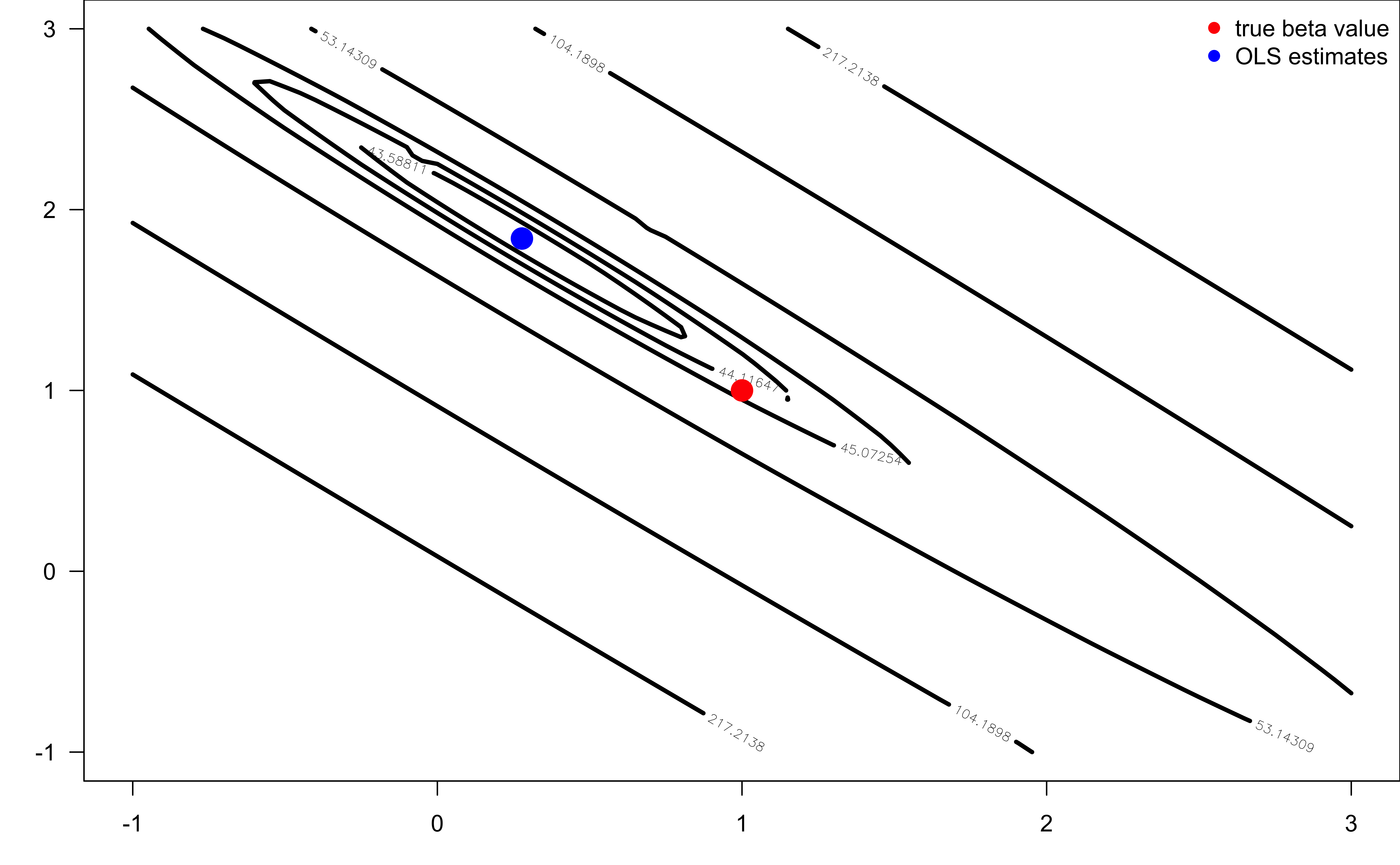
• \(\beta_1 = \beta_2 = 1\) and \(\mathrm{Corr}(x_1, x_2) = 0.99\)

• The relatively “flat” valley in the objective function walks along the eigen-vector of \({\bf X}'{\bf X}\) having the smallest eigen-value.

eigen(
    matrix(c(1, 0.99, 0.99, 1), 
             2, 2)
    )

eigen() decomposition
$values
[1] 1.99 0.01

$vectors
      [,1]   [,2]
[1,] 0.707 -0.707
[2,] 0.707  0.707

• From optimization point of view, the objective function (\(\ell_2\) loss) is “flat” along certain directions in the parameter domain.
• a small eigen-value in XTX makes the corresponding eigen-value large in the inverse.

Ridge and Valley

• Statisticians used to maximize the likelihood, leading to a “ridge”.

• Computer scientists like to minimize the loss, leading to a “valley”.

https://stats.stackexchange.com/questions/151304/why-is-ridge-regression-called-ridge-why-is-it-needed-and-what-happens-when

https://stats.stackexchange.com/questions/118712/why-does-ridge-estimate-become-better-than-ols-by-adding-a-constant-to-the-diago/119708#119708

When OLS Doesn’t Work Well: Optimization Perspective

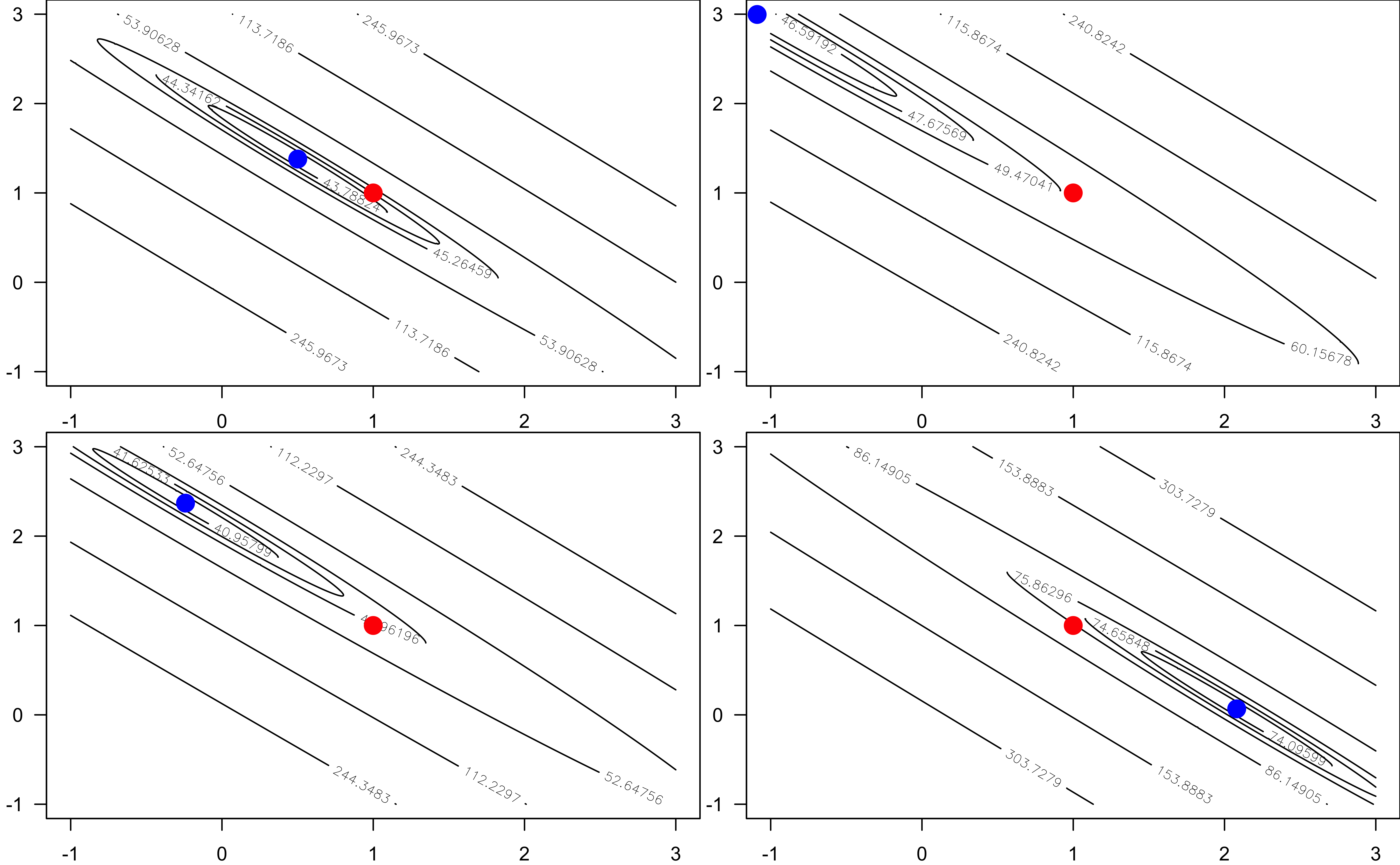
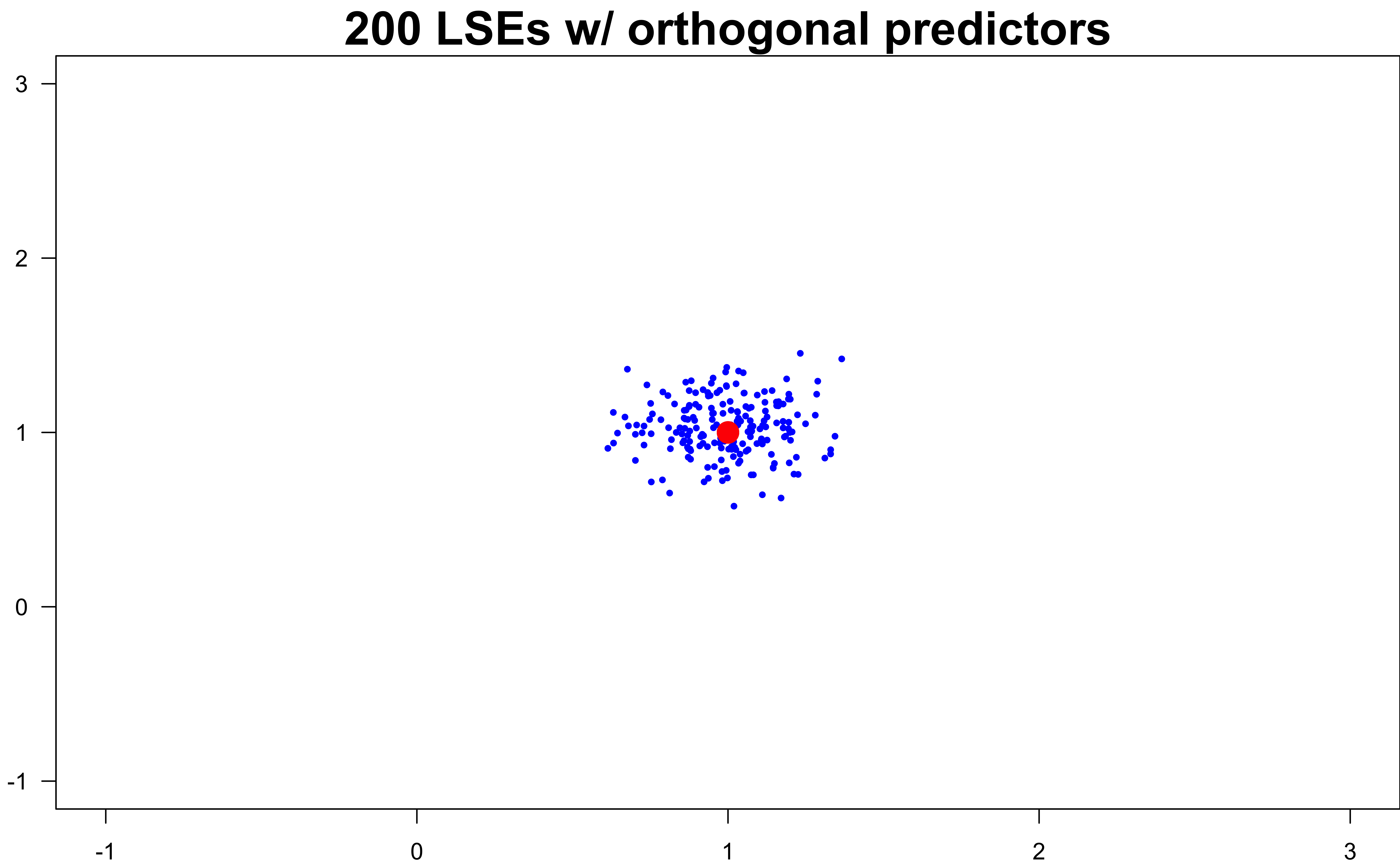
• A little change in the training set perturbs the objective function. The LSEs lie on a valley centered around the truth.

When OLS Doesn’t Work Well: High Variance

• The optimizer could land anywhere along the valley, leading to large variance of the LSE.

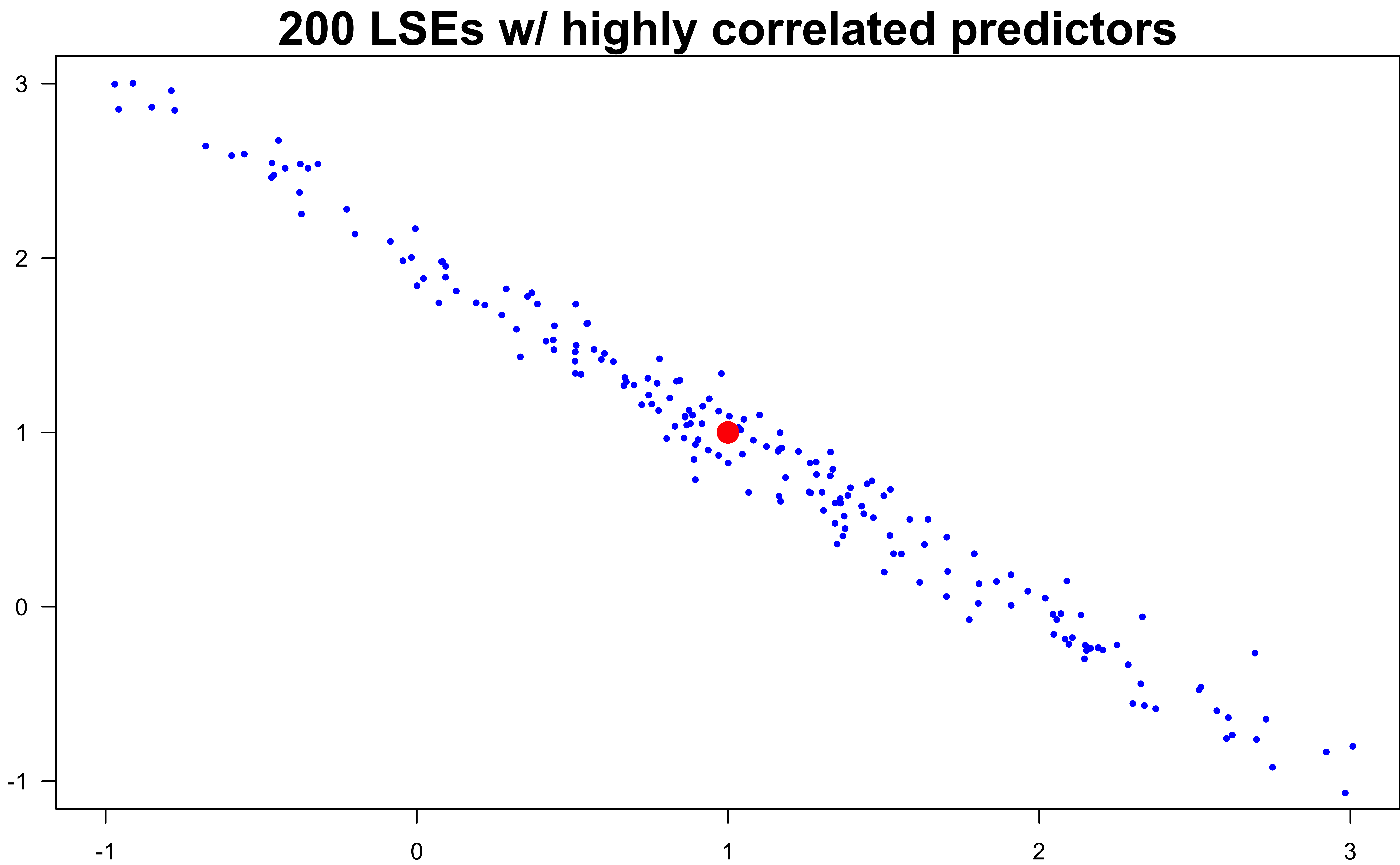
• Over many simulation runs, the LSE lies around the line of \(\beta_1 + \beta_2 = 2\), the direction of the eigen-vector of the smallest eigen-value.

The shape of the loss function for independent predictors is shown in 04-lin-reg optimization

When OLS Doesn’t Work Well: Large-\(p\)-small-\(n\) (High Dimensional Data)

• OLS stays well in the world of “large-\(n\)-small-\(p\)”.

• When \(p > n\), \({\bf X}'{\bf X}\) is not invertible.

• There is no unique \(\boldsymbol \beta\) estimate.

Intuition: Too many degrees of freedom (\(p\)) to specify a model, but not enough information (\(n\)) to decide which one is the one.

• Too flexible and ends up with overfitting

Too much flexibility about how \(f\) can be shaped, but too little information to guide or determine which shape it should be.

Remedy for Large Variance and Large-\(p\)-small-\(n\)

• Make \({\bf X}'{\bf X}\) invertible when \(p > n\) by regularizing coefficient behavior!

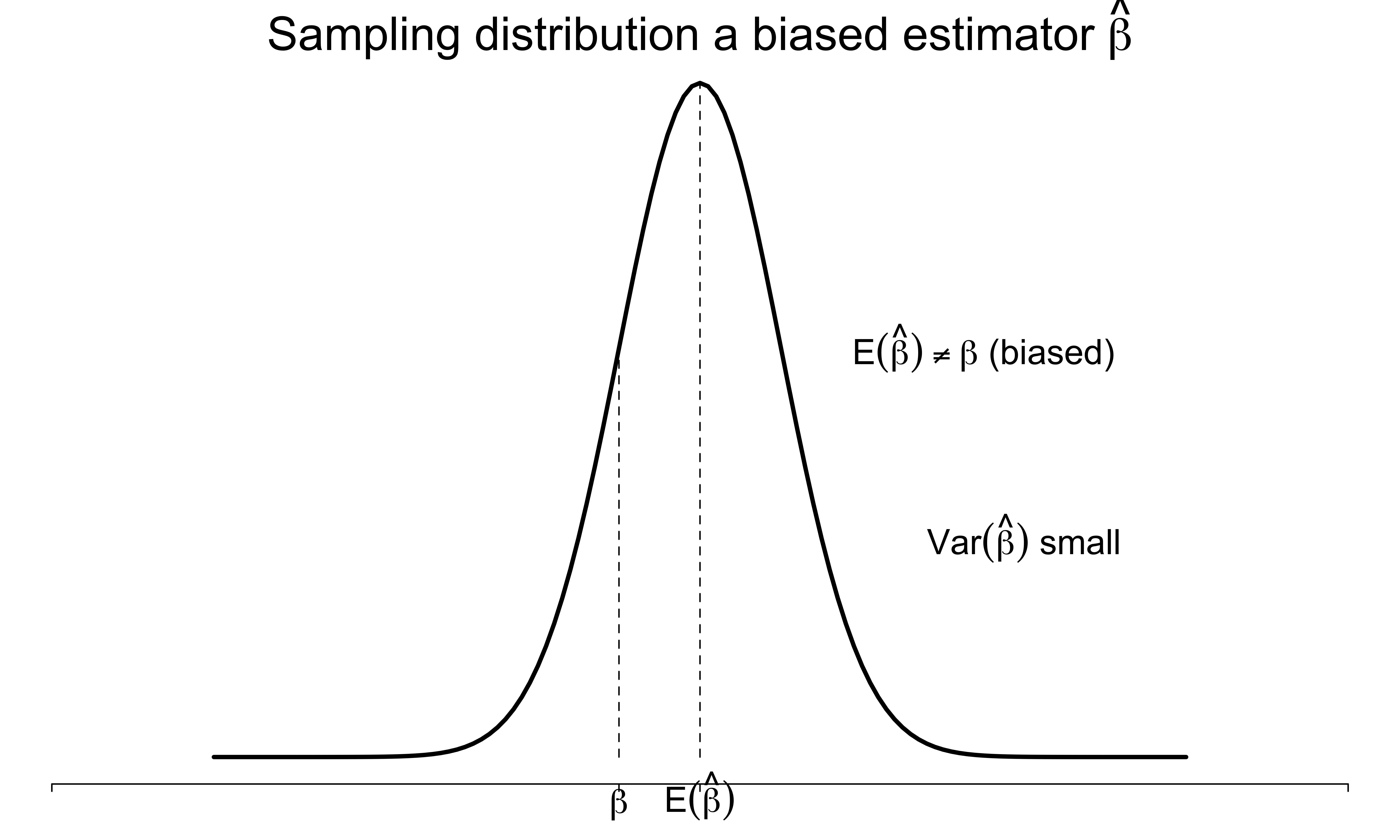
• A good estimator balances bias and variance well, or minimizes the mean square error \[\text{MSE}(\hat{\beta}) = E[(\hat{\beta} - \beta)^2] = \mathrm{Var}(\hat{\beta}) + \text{Bias}(\hat{\beta})^2\]

• A slightly biased estimator \(\hat{\boldsymbol \beta}\) that has much smaller variance and MSE than the LSE \({\bf b}\).

Ridge Regression

• Idea: Add a ridge (diagonal matrix) to \({\bf X} ' {\bf X}\).¹ \[\widehat{\boldsymbol \beta}^\text{r} = (\mathbf{X}' \mathbf{X}+ n \lambda \mathbf{I})^{-1} \mathbf{X}' \mathbf{y},\]

• To regularize coefficients, add an \(\ell_2\) penalty to the residual sum of squares, for some tuning parameter \(\lambda > 0\).

\[ \begin{align} \widehat{\boldsymbol \beta}^\text{r} =& \, \mathop{\mathrm{arg\,min}}_{\boldsymbol \beta} \underbrace{\lVert \mathbf{y}- \mathbf{X}\boldsymbol \beta\rVert_2^2}_{SS_{res}} + n \lambda \lVert\boldsymbol \beta\rVert_2^2\\ =& \, \mathop{\mathrm{arg\,min}}_{\boldsymbol \beta} \underbrace{\frac{1}{n} \sum_{i=1}^n (y_i - x_i'\boldsymbol \beta)^2}_{\text{MSE}_{\texttt{Tr}}} + \lambda \sum_{j=1}^p \beta_j^2\\ =& \, \mathop{\mathrm{arg\,min}}_{\boldsymbol \beta} \color{green} - \text{ goodness of fit } + \text{ model complexity/flexibility} \end{align} \]

1. This is a special case of the Tikhonov regularization.

Properties of Ridge Regression

\[ \begin{align} \widehat{\boldsymbol \beta}^\text{r} =& \mathop{\mathrm{arg\,min}}_{\boldsymbol \beta} \frac{1}{n} \sum_{i=1}^n (y_i - x_i'\boldsymbol \beta)^2 + \lambda \sum_{j=1}^p \beta_j^2, \end{align} \]

Properties of ridge regression:

• Has less degrees of freedom in the sense that the cost gets higher when larger coefficients are used.

• Favors small-magnitude coefficient estimates (Shrinkage) to avoid cost penalty.

• The shrinkage parameter \(\lambda\) controls the degree of penalty.
  • \(\lambda \rightarrow 0\): No penalty, and \(\widehat{\boldsymbol \beta}^\text{r} = \bf b\).
  • \(\lambda \rightarrow \infty\): Unbearable penalty, and \(\widehat{\boldsymbol \beta}^\text{r} \rightarrow \mathbf{0}\)

Ridge Penalty

\[\lambda \lVert \boldsymbol \beta\rVert^2_2 = \lambda \boldsymbol \beta' \mathbf{I}\boldsymbol \beta\]

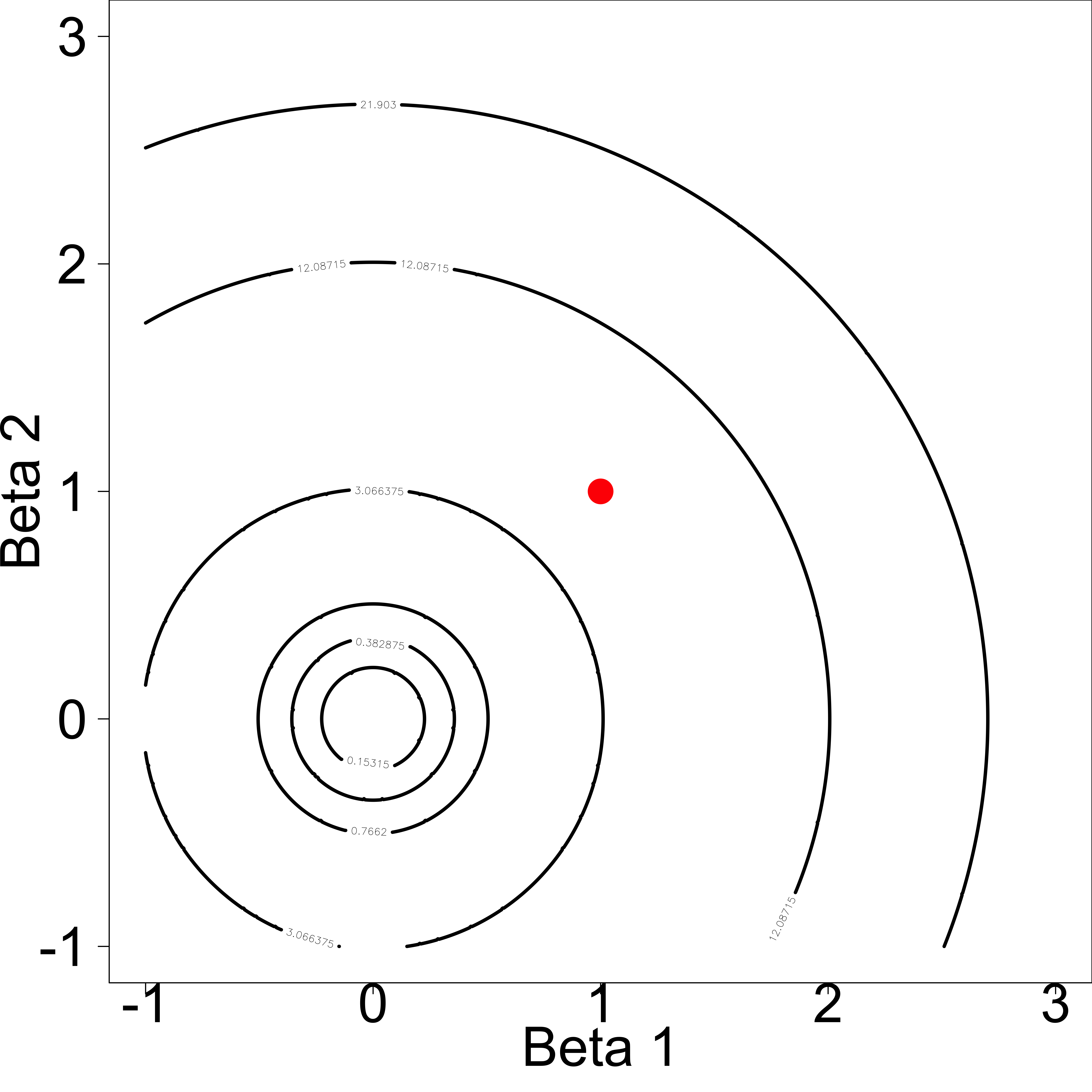
• The penalty contour is circle-shaped

• Force the objective function to be more convex

• A more stable or less varying solution

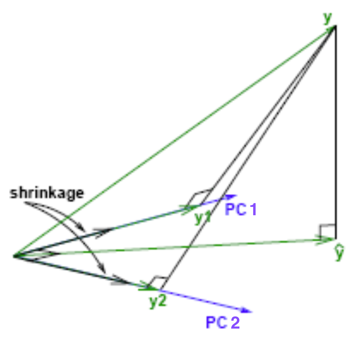
Geometrical Meaning of Ridge Regression

Source: https://online.stat.psu.edu/stat508/lessons/Lesson06

• Perform PCA of X
• Project y onto the PCs
• Shrinks the projection
• Reassemble the PCs using all the shrunken length

More Convex Loss Function

• Adding a ridge penalty forces the objective to be more convex due to the added eigenvalues.

eigen(matrix(c(1, 0.99, 0.99, 1), 2, 2) + diag(2))[1]

$values
[1] 2.99 1.01

Hence, by adding this to the OLS objective function, the solution is more stable, in the sense that each time we observe a new set of data, this contour looks pretty much the same. This may be interpreted in several different ways such as: 1) the objective function is more convex and less affected by the random samples; 2) the variance of the estimator is smaller because the eigenvalues of \(\mathbf{X}^\text{T}\mathbf{X}+ n \lambda \mathbf{I}\) are large.

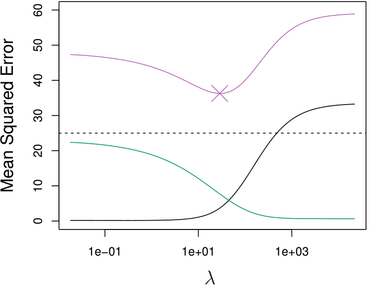
The Bias-variance Tradeoff

• As \(\lambda \downarrow\), bias \(\downarrow\) and variance \(\uparrow\)
• As \(\lambda \uparrow\), bias \(\uparrow\) and variance \(\downarrow\)

This effect is gradually changing as we increase the penalty level. The following simulation shows how the variation of \(\boldsymbol \beta\) changes. We show this with two penalty values, and see how the estimated parameters are away from the truth.

Now, we may ask the question: is it worth it? In fact, this bias and variance will be then carried to the predicted values \(x^\text{T}\widehat{\boldsymbol \beta}^\text{ridge}\). Hence, we can judge if this is beneficial from the prediction accuracy. And we need some procedure to do this.

Remark: The bias-variance trade-off will appear frequently in this course. And the way to evaluate the benefit of this is to see if it eventually reduces the prediction error (\(\text{Bias}^2 + \text{Variance}\) plus a term called irreducible error, which will be introduced in later chapter).

Lower Test MSE

• When \(b_j\) has large variance or \(p > n\), ridge regression could have lower test MSE and better predictive performance.

• \(\text{MSE}_{\texttt{Tr}}\) (purple)

• Squared bias (black)

• Variance (green)

Source: ISL Figure 6.5

MASS::lm.ridge()

• The lambda parameter in MASS::lm.ridge() specifies the \(n\lambda\) in our notation.

• OLS is scale equivalent: \(X_jb_j\) remains the same regardless of how \(X_j\) is scaled.

• Ridge coefficient estimates can change substantially when multiplying a given predictor by a constant, i.e., \(X_j\hat{\beta}^{r}_{j, \lambda}\) depends on \(\lambda\), the scaling of \(X_j\), and even the scaling of other predictors.

• Standardize all predictors!¹

head(mtcars, 3)

               mpg cyl disp  hp drat   wt qsec vs am gear carb
Mazda RX4     21.0   6  160 110 3.90 2.62 16.5  0  1    4    4
Mazda RX4 Wag 21.0   6  160 110 3.90 2.88 17.0  0  1    4    4
Datsun 710    22.8   4  108  93 3.85 2.32 18.6  1  1    4    1

(fit <- MASS::lm.ridge(mpg ~ ., data = mtcars, lambda = 1)) ## ridge fit

              cyl     disp       hp     drat       wt     qsec       vs 
16.53766 -0.16240  0.00233 -0.01493  0.92463 -2.46115  0.49259  0.37465 
      am     gear     carb 
 2.30838  0.68572 -0.57579 

1. In practice, if the intercept is not our interest, we also standardize the response.

Scaling of lm.ridge()

• coef(fit) transforms these back to the original scale for non-standardized \(\mathbf{X}\).

• fit$coef shows the coefficients of the standardized predictors.

coef(fit)

              cyl     disp       hp     drat       wt     qsec       vs 
16.53766 -0.16240  0.00233 -0.01493  0.92463 -2.46115  0.49259  0.37465 
      am     gear     carb 
 2.30838  0.68572 -0.57579 

fit$coef

   cyl   disp     hp   drat     wt   qsec     vs     am   gear   carb 
-0.285  0.285 -1.008  0.487 -2.370  0.866  0.186  1.134  0.498 -0.915 

Ridge Trace

ridge_fit <- lm.ridge(mpg ~ ., data = mtcars, lambda = 0:40)
matplot(coef(ridge_fit)[, -1], type = "l", xlab = "Lambda", ylab = "Coefficients")
text(rep(1, 10), coef(ridge_fit)[1,-1], colnames(mtcars)[2:11])

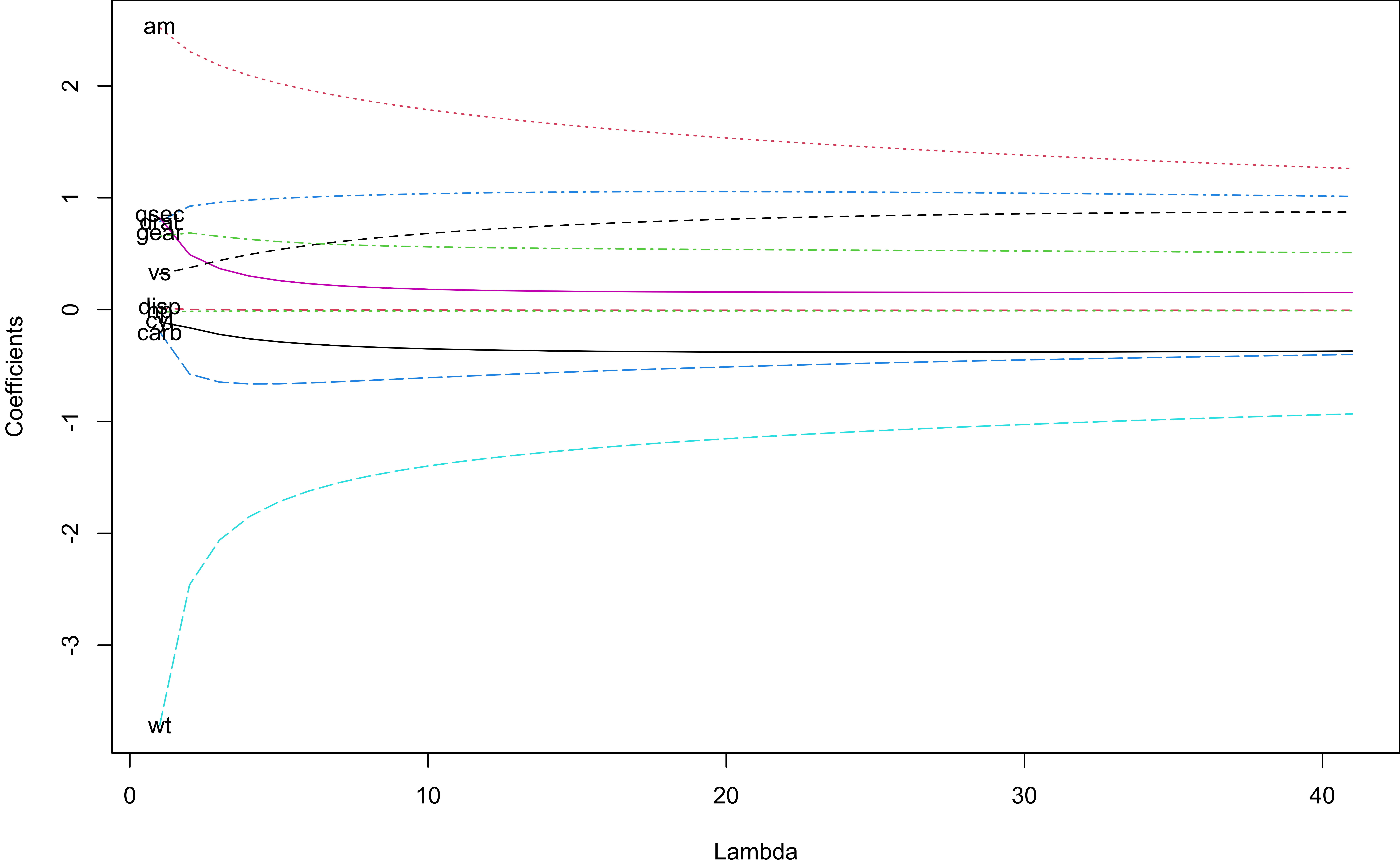
• Select a value of \(\lambda\) at which the ridge estimates are stable.

Methods for Choosing \(\lambda\)

MASS::select(ridge_fit)

modified HKB estimator is 2.59 
modified L-W estimator is 1.84 
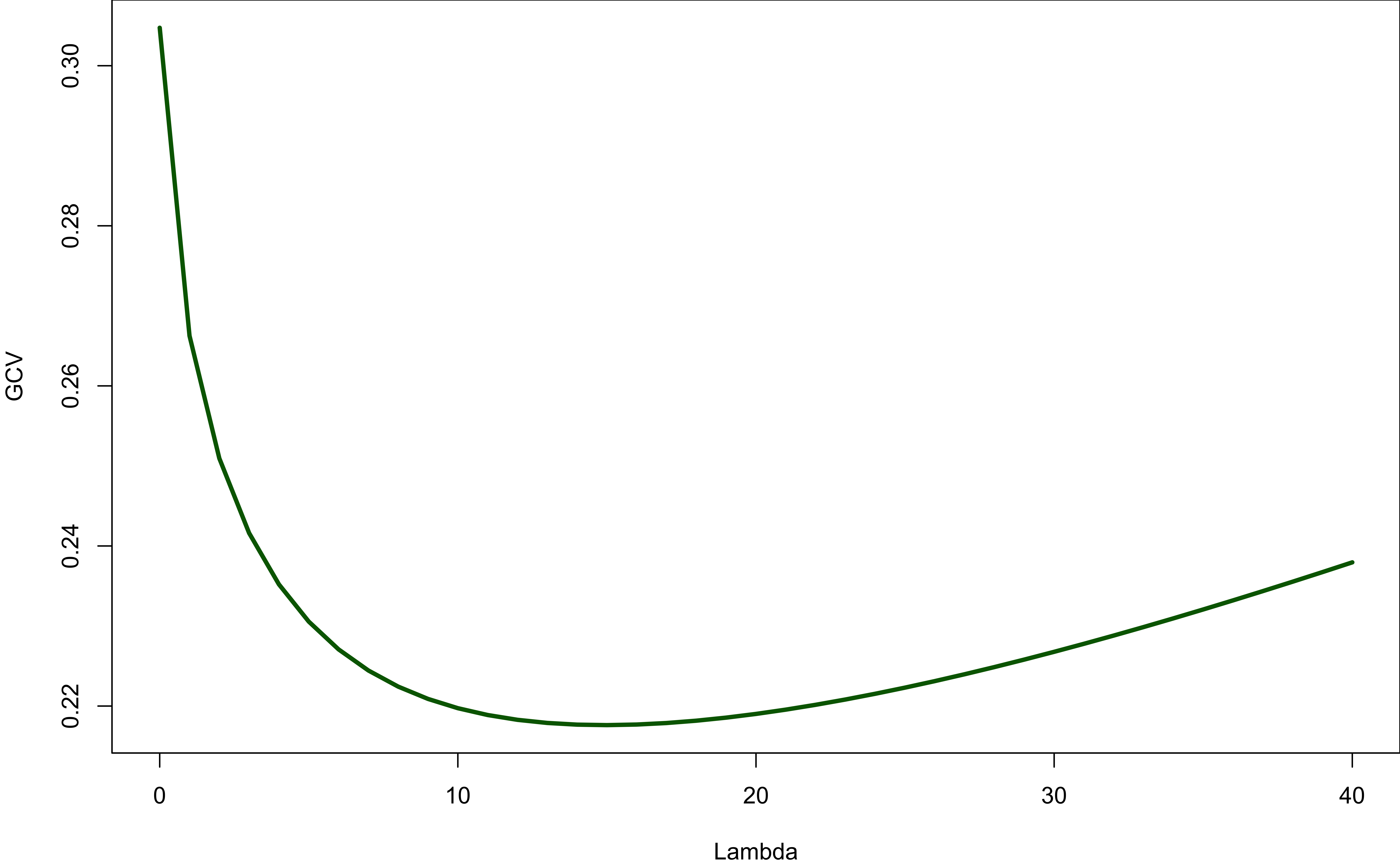
smallest value of GCV  at 15 

• Hoerl, Kennard, and Baldwin (1975): \(\lambda \approx \frac{p \hat{\sigma}^2}{{\bf b}'{\bf b}}\)

• Lawless and Wang (1976): \(\lambda \approx \frac{np \hat{\sigma}^2}{{\bf b'X}'{\bf Xb}}\)

• Golub, Health, and Wahba (1979): Generalized Cross Validation

Cross Validation

• Cross Validation (CV) is a resampling method.

• Resampling methods refit a model of interest to data sampled from the training set.

• CV can be used to

  • estimate the test error when there is no test data. (Model assessment)
  • select the tuning parameters that controls the model complexity/flexibility. (Model selection)

Hence, by adding this to the OLS objective function, the solution is more stable, in the sense that each time we observe a new set of data, this contour looks pretty much the same. This may be interpreted in several different ways such as: 1) the objective function is more convex and less affected by the random samples; 2) the variance of the estimator is smaller because the eigenvalues of \(\mathbf{X}^\text{T}\mathbf{X}+ n \lambda \mathbf{I}\) are large.

\(k\)-Fold Cross Validation

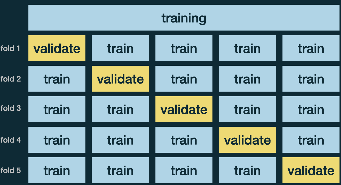
1. Randomly divide the training set into \(k\) folds, of approximately equal size.

2. Use 1 fold for validation to compute MSE, and the remaining \(k - 1\) partitions for training.

3. Repeat \(k\) times. Each time a different fold is treated as a validation set.

4. Average \(k\) metrics, \(\text{MSE}_{CV} = \frac{1}{k}\sum_{i=1}^k\text{MSE}_i\).

5. Use the CV estimate \(\text{MSE}_{CV}\) to select the “best” tuning parameter.

Five-fold cross validation. Source: Data science in a box

Can compute other performance measures.

glmnet package

• The parameter alpha controls the ridge (alpha = 0) and lasso (alpha = 1) penalties.

• Supply a decreasing sequence of lambda values.

• lm.ridge() use \(SS_{res}\) and \(n\lambda\), while glmnet() use \(\text{MSE}_{\texttt{Tr}}\) and \(\lambda\).

• Argument x should be a matrix.

glmnet(x = data.matrix(mtcars[, -1]), 
       y = mtcars$mpg, 
       alpha = 0, 
       lambda = 5:0/nrow(mtcars))

lm.ridge(formula = mpg ~ ., 
         data = mtcars, 
         lambda = 5:0)

Note

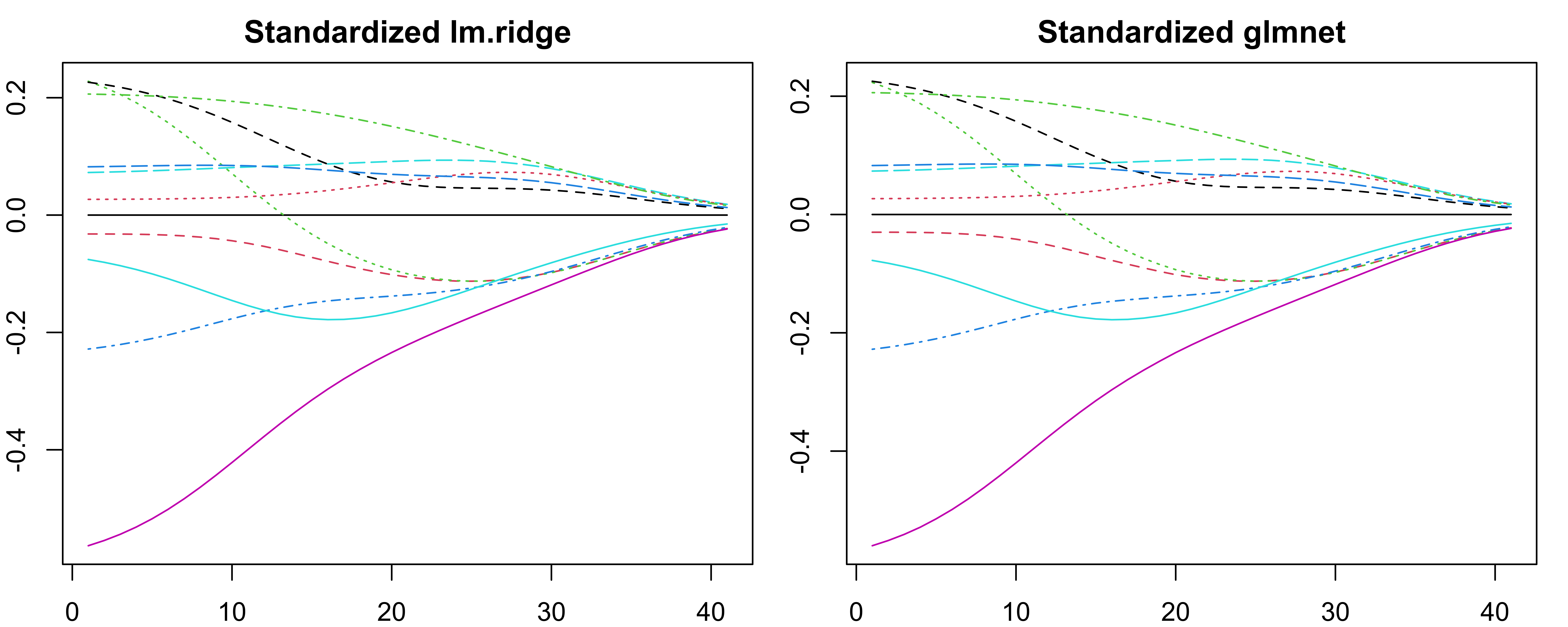
• glmnet() only use coef() and return coefficients at the original scale.

• lm.ridge() and glmnet() coefficients do not match exactly, especially when transforming back to original scale.

• No need to worry too much as we focus on predictive performance.

https://stats.stackexchange.com/questions/74206/ridge-regression-results-different-in-using-lm-ridge-and-glmnet

by default, glmnet standardize predictors and include intercept

\(k\)-Fold Cross Validation using cv.glmnet()¹

• The \(\lambda\) values are automatically selected, on the \(\log_{e}\) scale.

ridge_cv_fit <- cv.glmnet(x = data.matrix(mtcars[, -1]), y = mtcars$mpg, alpha = 0,
                          nfolds = 10, type.measure = "mse")
plot(ridge_cv_fit$glmnet.fit, "lambda")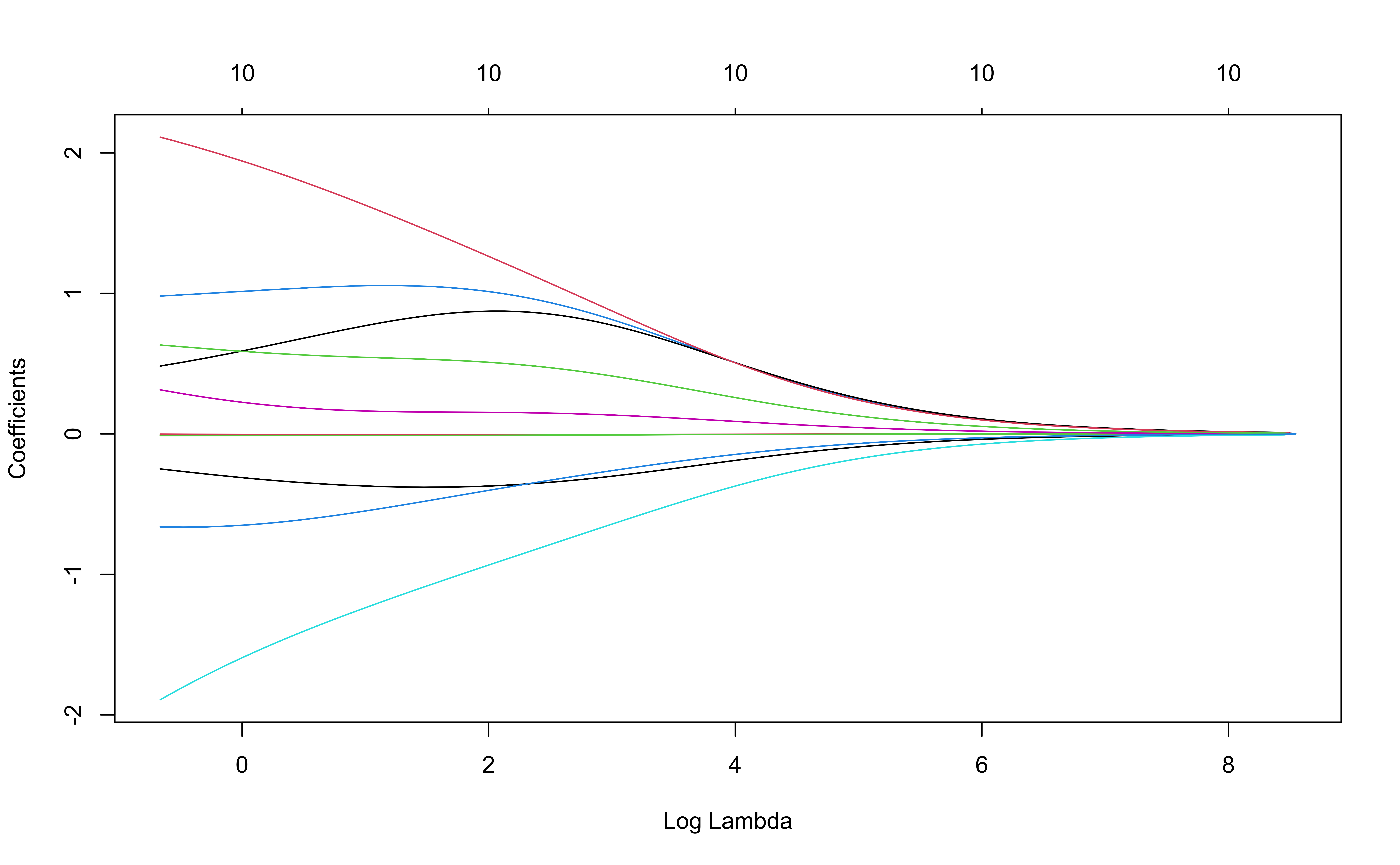

• Why s and not lambda? In case we want to allow one to specify the model size in other ways in the future. s: Value(s) of the penalty parameter lambda at which predictions are required. Default is the entire sequence used to create the model.

1. There are other ways to do CV for ridge regression in R, for example, the caret (Classification And REgression Training) package and the rsample package in tidymodels ecosystem.

Determine \(\lambda\)

plot(ridge_cv_fit)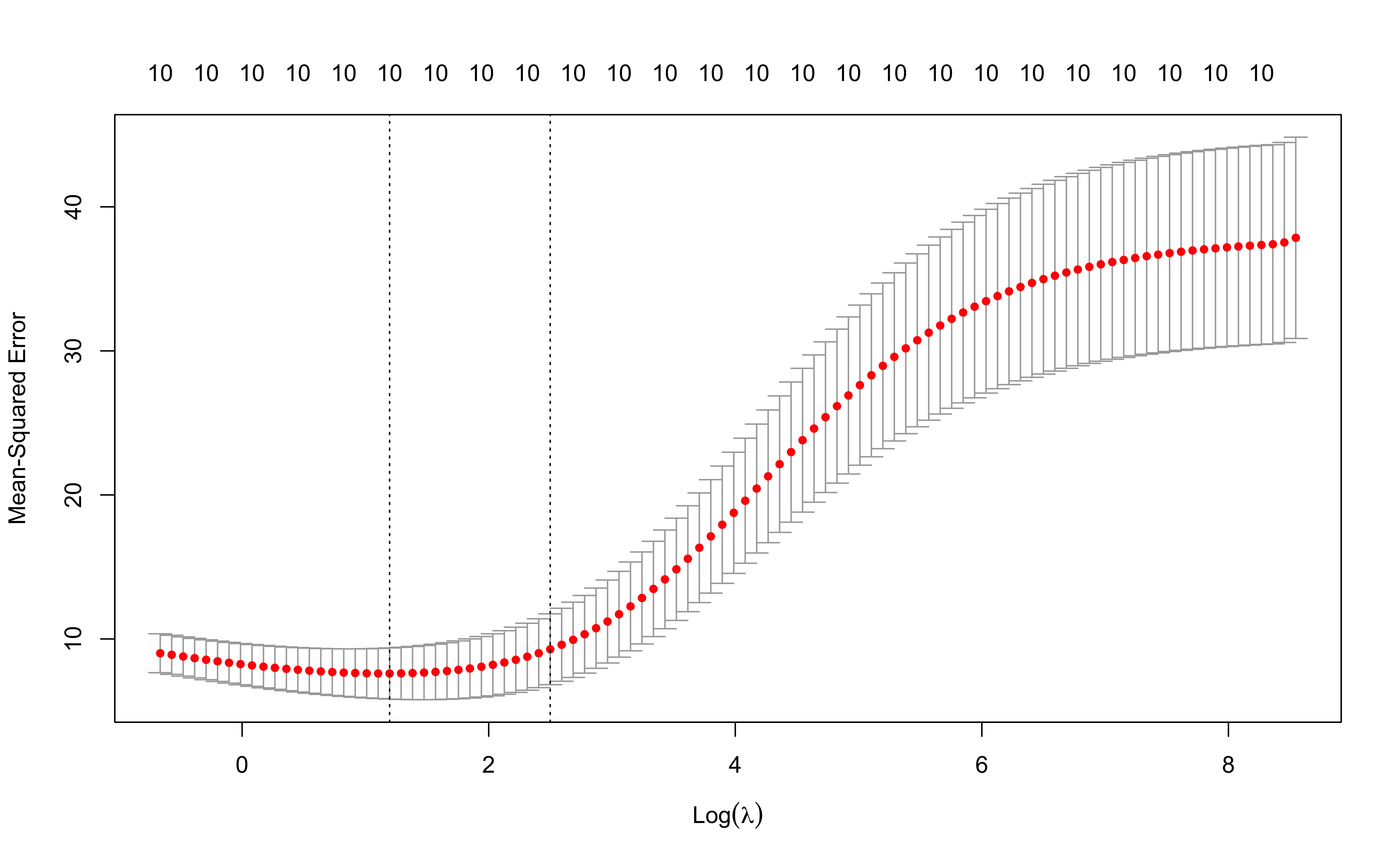

ridge_cv_fit$lambda.min

[1] 3.31

# largest lambda s.t. error is within 1 s.e of the min
ridge_cv_fit$lambda.1se 

[1] 12.2

coef(ridge_cv_fit, s = "lambda.min")

11 x 1 sparse Matrix of class "dgCMatrix"
                  s1
(Intercept) 20.97465
cyl         -0.37636
disp        -0.00537
hp          -0.01139
drat         1.05572
wt          -1.17533
qsec         0.15874
vs           0.80136
am           1.55883
gear         0.53942
carb        -0.52151

coef(fit2, s = “lambda.1se”) This plots the cross-validation curve (red dotted line) along with upper and lower standard deviation curves along the 𝜆 sequence (error bars). Two special values along the 𝜆 sequence are indicated by the vertical dotted lines. lambda.min is the value of 𝜆 that gives minimum mean cross-validated error, while lambda.1se is the value of 𝜆 that gives the most regularized model such that the cross-validated error is within one standard error of the minimum. https://stats.stackexchange.com/questions/253963/how-to-interpret-cv-glmnet-plot

Generalized Cross-Validation

• The generalized cross-validation (GCV) is a modified version of the leave-one-out CV (LOOCV) (\(n\)-fold CV).

• The LOOCV for linear regression is

\[\text{CV}_{(n)} = \frac{1}{n}\sum_{i=1}^n \left[ \frac{y_i - x_i' {\mathbf{b}}} {1 - {\bf H}_{ii}} \right]^2 \]

• The GCV criterion is given by

\[\text{GCV}(\lambda) = \frac{1}{n}\sum_{i=1}^n \left[ \frac{y_i - x_i' \widehat{\boldsymbol \beta}^\text{r}_\lambda}{1 - \frac{\text{Trace}(\mathbf{S}_\lambda)}{n}} \right]^2\]

where \(\mathbf{S}_\lambda\) is the hat matrix corresponding to the ridge regression:

\[\mathbf{S}_\lambda = \mathbf{X}(\mathbf{X}' \mathbf{X}+ n\lambda \mathbf{I})^{-1} \mathbf{X}'\]

The interesting fact about leave-one-out CV in the linear regression setting is that we do not need to explicitly fit all leave-one-out models.

• ESL p. 244

• lm.ridge code

Generalized Cross-Validation

Select the best \(\lambda\) that produces the smallest GCV error.

ridge_fit <- lm.ridge(mpg ~ ., data = mtcars, lambda = 0:40)

plot(ridge_fit$lambda, 
     ridge_fit$GCV, 
     type = "l", col = "darkgreen", 
     ylab = "GCV", xlab = "Lambda", 
     lwd = 3)

idx <- which.min(ridge_fit$GCV)
ridge_fit$lambda[idx]

[1] 15

round(coef(ridge_fit)[idx, ], 2)

        cyl  disp    hp  drat    wt  qsec    vs    am  gear  carb 
21.13 -0.37 -0.01 -0.01  1.05 -1.23  0.16  0.77  1.62  0.54 -0.55 

You can clearly see that the GCV decreases initially, as \(\lambda\) increases, this is because the reduced variance is more beneficial than the increased bias. However, as \(\lambda\) increases further, the bias term will eventually dominate and causing the overall prediction error to increase. The fitted MSE under this model is