Bayesian Inference and Linear Regression

MSSC 6250 Statistical Machine Learning

Dr. Cheng-Han Yu
Department of Mathematical and Statistical Sciences
Marquette University

Bayesian Inference*

Thinking like a Bayesian

1. When flipping a fair coin, we say that “the probability of flipping Heads is 0.5.” How do you interpret this probability?

   1. If I flip this coin over and over, roughly 50% will be Heads.
   2. Heads and Tails are equally plausible.
   3. Both a. and b. make sense.

2. An election is coming up and a pollster claims that candidate Yu has a 0.9 probability of winning. How do you interpret this probability?

   1. If we observe the election over and over, candidate Yu will win roughly 90% of the time.
   2. Candidate Yu is much more likely to win than to lose.
   3. The pollster’s calculation is wrong. Candidate Yu will either win or lose, thus their probability of winning can only be 0 or 1.

• 1. a = 1 pt, b = 3 pts, c = 2 pts
• 2. a = 1 pt, b = 3 pts, c = 1 pt

Thinking like a Bayesian

3. Two claims.

   (1) Ben claims he can predict the coin flip outcome. To test his claim, you flip a fair coin 8 times and he correctly predicts all.

   (2) Emma claims she can distinguish natural and artificial sweeteners. To test her claim, you give her 8 samples and she correctly identifies each.

   In light of these experiments, what do you conclude?

   1. You’re more confident in Emma’s claim than Ben’s claim.
   2. The evidence supporting Ben’s claim is just as strong as the evidence supporting Emma’s claim.

4. Suppose that during a doctor’s visit, you tested positive for COVID. If you only get to ask the doctor one question, which would it be?

   1. What’s the chance that I actually have COVID?
   2. If in fact I don’t have COVID, what’s the chance that I would’ve gotten this positive test result?

• 3. a = 3 pts, b = 1 pt
• 4. a = 3 pts, b = 1 pt

Totals from 4–5 indicate that your current thinking is fairly frequentist, whereas totals from 9–12 indicate alignment with the Bayesian philosophy. In between these extremes, totals from 6–8 indicate that you see strengths in both philosophies.

Frequentist or Bayesian?

• Totals 4-5: your thinking is frequentist

• Totals 9-12: your thinking is Bayesian

• Totals 6-8: you see strengths in both philosophies

The Meaning of Probability: Relative Frequency

• The frequentist interprets probability as the long-run relative frequency of a repeatable experiment.

The probability that some outcome of a process will be obtained is defined as

the relative frequency with which that outcome would be obtained if the process were repeated a large number of times independently under similar conditions.

      Frequency Relative Frequency
Heads         4                0.4
Tails         6                0.6
Total        10                1.0
---------------------
      Frequency Relative Frequency
Heads       512              0.512
Tails       488              0.488
Total      1000              1.000
---------------------

• If we repeat tossing the coin 10 times, the probability of obtaining heads is 40%.
• If 1000 times, the probability is 51.2%.

source: usplash

Issues of Relative Frequency

• 😕 How large of a number is large enough?

• 😕 Meaning of “under similar conditions”

• 😕 The relative frequency is reliable under identical conditions?

• 👉 We only obtain an approximation instead of exact value.

• 😂 How do you compute the probability that Chicago Cubs wins the World Series next year?

The Meaning of Probability: Relative Plausibility

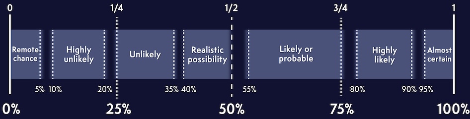
• In the Bayesian philosophy, a probability measures the relative plausibility of an event.

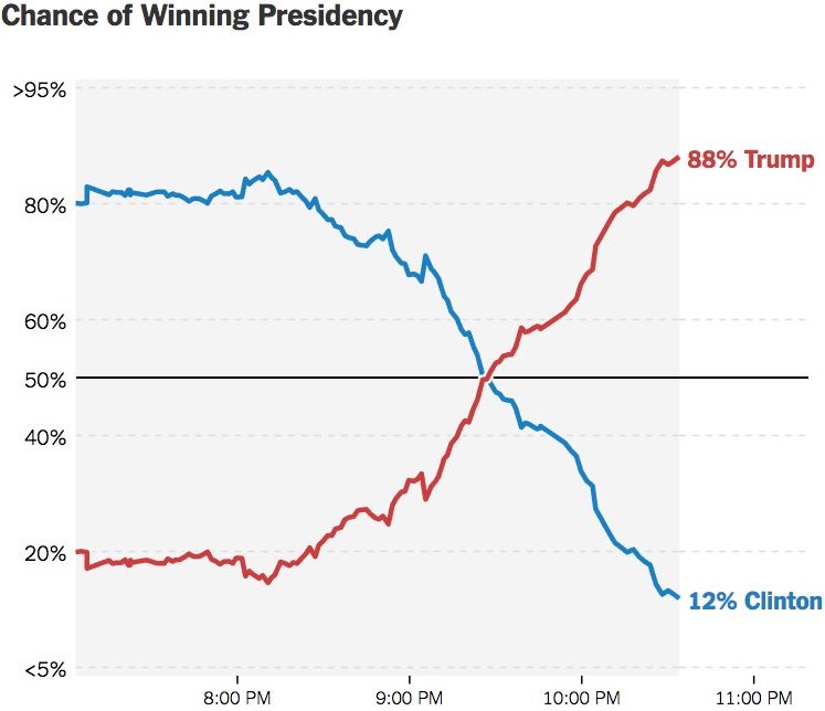
• For the statement “candidate A has a 0.9 probability of winning”
  • A frequentist might say
    1. the conclusion is wrong
    2. (weirdly) in long-run hypothetical repetitions of the election, candidate A would win roughly 90% of the time.
  • A Bayesian would say based on analysis the candidate A is 9 times more likely to win than to lose.

Source: https://twitter.com/nytgraphics/status/796195155158171648/photo/1

• For the statement “the probability of flipping Heads is 0.5”
  • A frequentist would conclude that if we flip the coin over and over, roughly 1/2 of these flips will be Heads.
  • A Bayesian would conclude that Heads and Tails are equally likely.

Your Degree of Uncertainty or Ignorance

Source: Defence Intelligence – communicating probability

• I’m gonna flip a coin, and ask you the probability it’ll come up heads. You say “50–50”.

• I then flip the coin, take a peek, but cover it up, and ask: what’s your probability it’s heads now?

• The event has happened, and no randomness left - just your ignorance!

David Spiegelhalter (2024). Why probability probably doesn’t exist (but it is useful to act like it does). Nature, 636, p. 560 - 563.

it handles both chance and ignorance.

I will argue — whether in a scientific paper, as part of weather forecasts, predicting the outcome of a sports competition or quantifying a health risk — is not an objective property of the world, but a construction based on personal or collective judgements and (often doubtful) assumptions. Furthermore, in most circumstances, it is not even estimating some underlying ‘true’ quantity. Probability, indeed, can only rarely be said to ‘exist’ at all.

To get a handle on probability’s slipperiness, consider how the concept is used in modern weather forecasts. Meteorologists make predictions of temperature, wind speed and quantity of rain, and often also the probability of rain — say 70% for a given time and place. The first three can be compared with their ‘true’ values; you can go out and measure them. But there is no ‘true’ probability to compare the last with the forecaster’s assessment. There is no ‘probability-ometer’. It either rains or it doesn’t.

There is another lesson in here. Even if there is a statistical model for what should happen, this is always based on subjective assumptions

My argument is that any practical use of probability involves subjective judgements. This doesn’t mean that I can put any old numbers on my thoughts — I would be proved a poor probability assessor if I claimed with 99.9% certainty that I can fly off my roof, for example. The objective world comes into play when probabilities, and their underlying assumptions, are tested against reality (see ‘How ignorant am I?’); but that doesn’t mean the probabilities themselves are objective.

Everybody Changes Their Mind

How can we live if we don’t change? - Beyoncé. Lyric from “Satellites.”

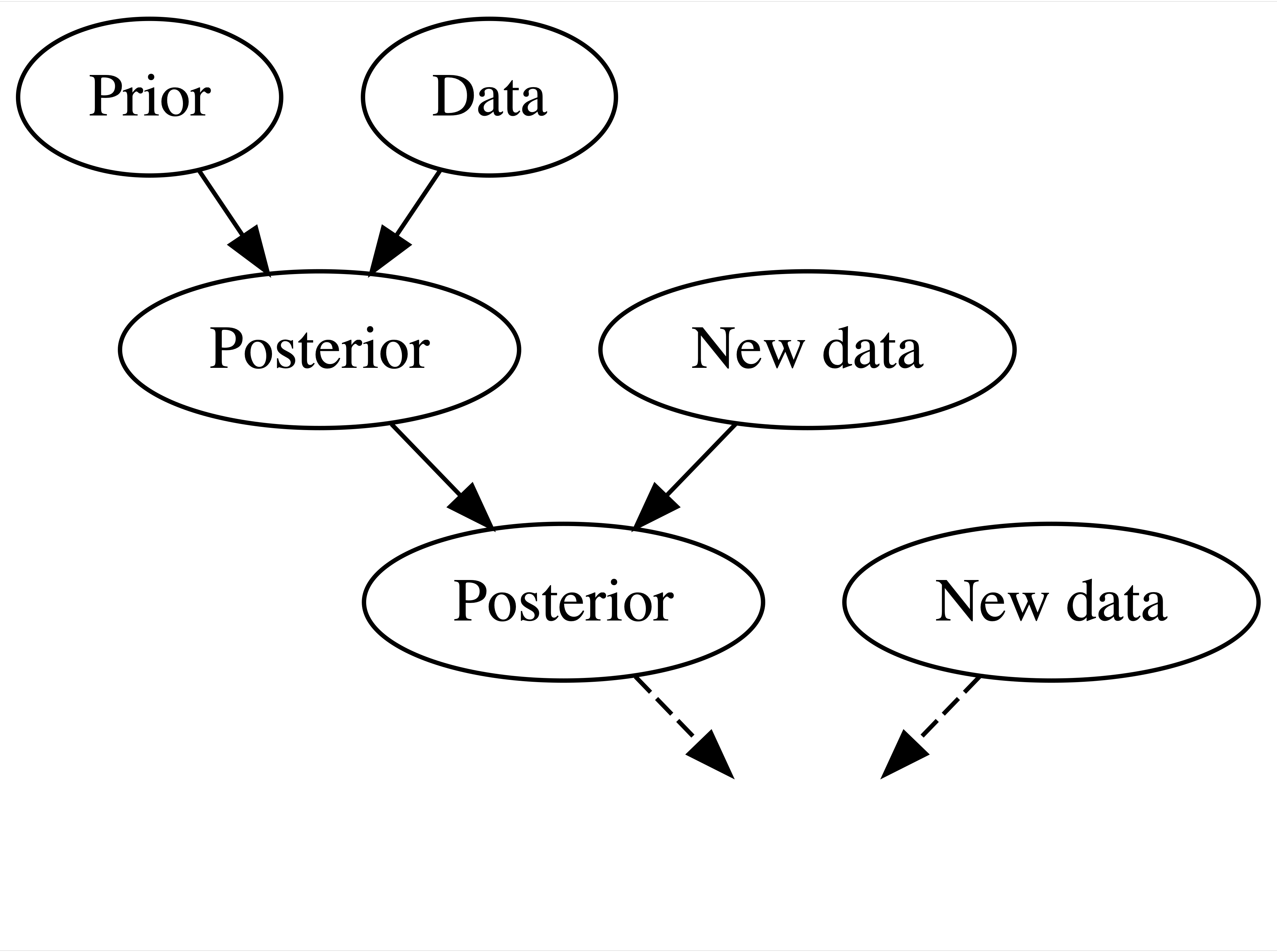
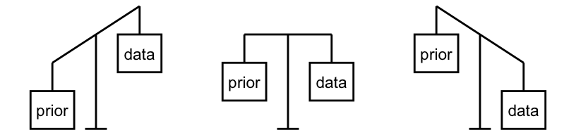
• Using data and prior beliefs to update our knowledge (posterior), and repeating.

• We continuously update our knowledge about the world as we accumulate lived experiences, or collect data.

Fig 1.1 of https://www.bayesrulesbook.com/. The figures not being sourced come from this book too.

Everybody changes their mind. You likely even changed your mind in the last minute. For example, suppose there’s a new Italian restaurant in your town. It has a 5-star online rating and you love Italian food! Thus, prior to ever stepping foot in the restaurant, you anticipate that it will be quite delicious. On your first visit, you collect some edible data: your pasta dish arrives a soggy mess. Weighing the stellar online rating against your own terrible meal (which might have just been a fluke), you update your knowledge: this is a 3-star not 5-star restaurant. Willing to give the restaurant another chance, you make a second trip. On this visit, you’re pleased with your Alfredo and increase the restaurant’s rating to 4 stars. You continue to visit the restaurant, collecting edible data and updating your knowledge each time.

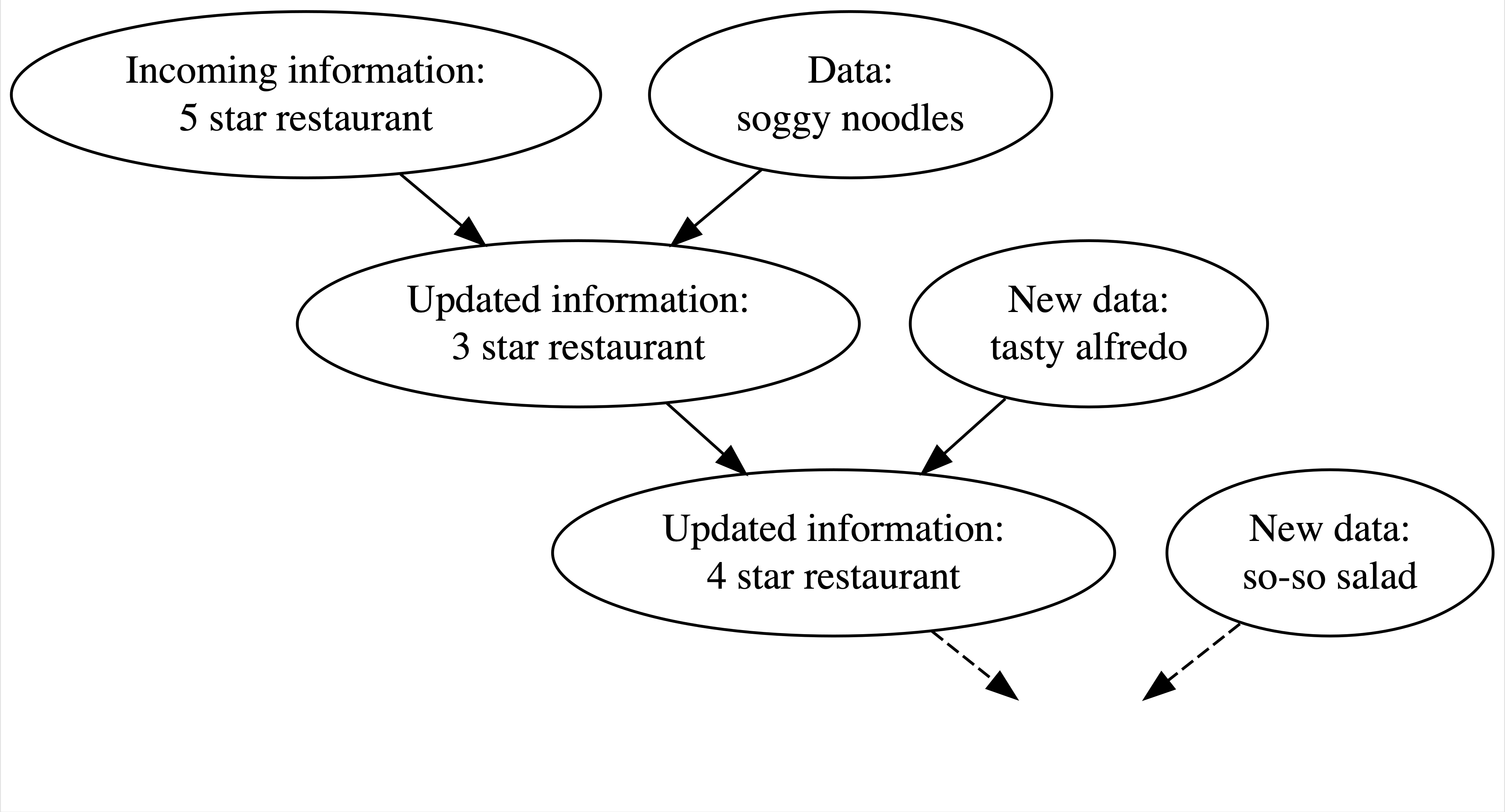
Bayesian Knowledge-building Process

If you’re an environmental scientist, yours might be an analysis of the human role in climate change. You don’t walk into such an inquiry without context – you carry a degree of incoming or prior information based on previous research and experience. Naturally, it’s in light of this information that you interpret new data, weighing both in developing your updated or posterior information.

Frequentist Relys on (Limited) Data Only

• In Question 3, in a frequentist analysis, “8 out of 8” is “8 out of 8” no matter if it’s in the context of Ben’s coins or Emma’s sweeteners.
  • Equally confident conclusions that Ben can predict coin flips and Emma can distinguish between natural and artificial sweeteners.

• But do you really believe Ben’s claim 100%? 🤔 😕

• In fact, we judge their claim before evidence are collected, don’t we? 🤔

• You probably think Ben overstates his ability but Emma’s claim sounds relatively reasonable, right?

The Bayesian Balancing

• Frequentist throws out all prior knowledge in favor of a mere 8 data points.

• Bayesian analyses balance and weight our prior experience/knowledge/belief and new data/evidence to judge a claim or make a conclusion.

• We are not stubborn! If Ben had correctly predicted the outcome of 1 million coin flips, the strength of this data would far surpass that of our prior judgement, leading to a posterior conclusion that perhaps Ben is psychic!

Seeing is believing

Asking Different Questions

In Question 4,

• Bayesians answer (a) what’s the chance that I actually have COVID?
• Frequentists answer (b) if in fact I do not have COVID, what’s the chance that I would’ve gotten this positive test result?

	Test Positive	Test Negative	Total
COVID	3	1	4
No COVID	9	87	96
Total	12	88	100

• \(H_0\): Do not have COVID vs. \(H_1\): Have COVID

• A frequestist assesses the uncertainty of the observed data in light of an assumed hypothesis \(P(Data \mid H_0) = 9/96\)

• A Bayesian assesses the uncertainty of the hypothesis in light of the observed data \(P(H_0 \mid Data) = 9/12\)

a Bayesian analysis would ask: Given my positive test result, what’s the chance that I actually have the disease? Since only 3 of the 12 people that tested positive have the disease (Table 1.1), there’s only a 25% chance that you have the disease. Thus, when we take into account the disease’s rarity and the relatively high false positive rate, it’s relatively unlikely that you actually have the disease. What a relief.

since disease status isn’t repeatable, the probability you have the disease is either 1 or 0 – you have it or you don’t. To the contrary, medical testing (and data collection in general) is repeatable. You can get tested for the disease over and over and over. Thus, a frequentist analysis would ask: If I don’t actually have the disease, what’s the chance that I would’ve tested positive? Since only 9 of the 96 people without the disease tested positive, there’s a roughly 10% (9/96) chance that you would’ve tested positive even if you didn’t have the disease.

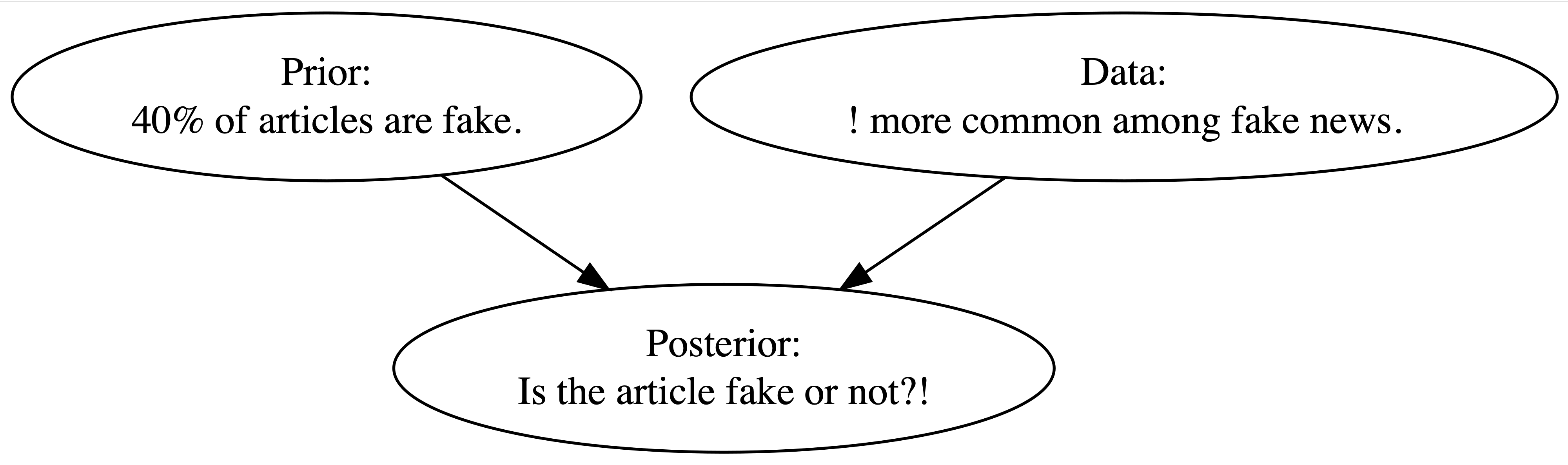
Fake News

• To do: Predict whether or not if an incoming article is fake.

• Prior info: 40% of the articles are fake

• Data come in: Check several fake and real articles, and found ! is more consistent with fake news (Evidence).

 title_has_excl fake real
          FALSE   44   88
           TRUE   16    2
          Total   60   90

The usage of an ! might seem odd for a real article. The exclamation point data is more consistent with fake news.

Bayesian Updating Rule

• \(F\): an article is fake.

• The prior probability model

Event	\(F\)	\(F^c\)	Total
Probability \(P(\cdot)\)	0.4	0.6	1

Bayesian Model for Events

 title_has_excl fake real
          FALSE   44   88
           TRUE   16    2
          Total   60   90

• \(D\): an article title has exclamation mark.

• Conditional probability: \(P(D \mid {\color{blue}{F}}) = 16/60 = 27\%\); \(P(D \mid {\color{blue}{F^c}}) = 2/90 = 2\%\).

• Opposite position:
  • Know the incoming article used ! (observed data \({\color{blue}{D}}\))
  • Don’t know whether or not the article is fake \(F\) (what we want to decide).

• Compare \(P(D \mid F)\) and \(P(D \mid F^c)\) to ascertain the relative likelihoods of observed data \({\color{blue}{D}}\) under different scenarios of the uncertain article status.

Since exclamation point usage is so much more likely among fake news than real news, this data provides some evidence that the article is fake To help distinguish this application of conditional probability calculations from that when
D is uncertain and F is known, we’ll utilize the following likelihood function notation.

Likelihood Function

• Likelihood function \(L(\cdot\mid {\color{blue}{D}})\):

\[L(F \mid {\color{blue}{D}}) = P({\color{blue}{D}} \mid F) \text{ and } L(F^c \mid {\color{blue}{D}}) = P({\color{blue}{D}} \mid F^c)\]

• When \({\color{blue}{F}}\) is known, the conditional probability function \(P(\cdot \mid {\color{blue}{F}})\) compares the probabilities of an unknown event \(D\), \(D^c\), occurring with \(F\): \[P(D \mid {\color{blue}{F}}) \text{ vs. } P(D^c \mid {\color{blue}{F}})\]

• When \({\color{blue}{D}}\) is known, the likelihood function \(L(\cdot \mid {\color{blue}{D}}) = P({\color{blue}{D}} \mid \cdot)\) evaluates the relative compatibility of data \(D\) with \(F\) or \(F^c\): \[L(F \mid {\color{blue}{D}}) \text{ vs. } L(F^c \mid {\color{blue}{D}})\]

Event	\(F\)	\(F^c\)	Total
Probability \(P(\cdot)\)	0.4	0.6	1
Likelihood \(L(\cdot \mid D)\)	0.27	0.02	0.29

• The likelihood function is not a probability function!

Bayes’ Rule

\[\begin{align*} P(F \mid D) &= \frac{P(F \cap D)}{P(D)}\\ &= \frac{L(F \mid D)P(F)}{P(D)}\end{align*}\]

\[\text{posterior = } \frac{\text{likelihood} \cdot \text{prior }}{ \text{normalizing constant}} \]

• The normalizing constant \(P(D)\) is known as marginal likelihood or evidence.

\[\begin{align*} P(F \mid D) &= \frac{P(F \cap D)}{P(D)}\\ &= \frac{P(D \mid F)P(F)}{P(D)} \\ &= \frac{P(D \mid F)P(F)}{P(D \mid F)P(F) + P(D \mid F^c)P(F^c)}\\ &= \frac{L(F \mid D)P(F)}{L(F \mid D)P(F) + L(F^c \mid D)P(F^c)}\end{align*}\]

Posterior

• Started with a prior understanding that there’s a 40% chance that the incoming article would be fake.

• Yet upon observing the use of an exclamation point in the title

“The president has a funny secret!”

a feature that’s more common to fake news.

• Our posterior understanding evolved quite a bit – the chance that the article is fake jumped to 89%.

Event	\(F\)	\(F^c\)	Total
Prior prob \(P(\cdot)\)	0.4	0.6	1
Posterior prob \(P(\cdot \mid D)\)	0.89	0.11	1

Bayesian Inference for Random Variables

For any random variables parameter \(\theta\) and data \({\bf Y} = (Y_1, \dots, Y_n)\),

• \(\pi(\theta)\): the prior pmf/pdf of \(\theta\)

• \(L(\theta \mid y_1,\dots, y_n)\): the likelihood of \(\theta\) given observed data \(\mathbf{y}= \{y_i \}_{i = 1}^n\).

• The posterior distribution of \(\theta\) given \(\mathbf{y}\) is

\[\pi(\theta \mid \mathbf{y}) = \frac{L(\theta \mid \mathbf{y})\pi(\theta)}{p(\mathbf{y})}\] where \[p(\mathbf{y}) = \begin{cases} \int_{\Theta} L(\theta \mid \mathbf{y})\pi(\theta) ~ d\theta & \text{if } \theta \text{ is continuous }\\ \sum_{\theta \in \Theta} L(\theta \mid \mathbf{y})\pi(\theta) & \text{if } \theta \text{ is discrete } \end{cases}\]

Proportionality

\[\pi(\theta \mid \mathbf{y}) = \frac{L(\theta \mid \mathbf{y})\pi(\theta)}{p(\mathbf{y})} \propto_{\theta} L(\theta \mid \mathbf{y})\pi(\theta)\]

\[\text{posterior } \propto \text{ likelihood } \cdot \text{ prior } \]

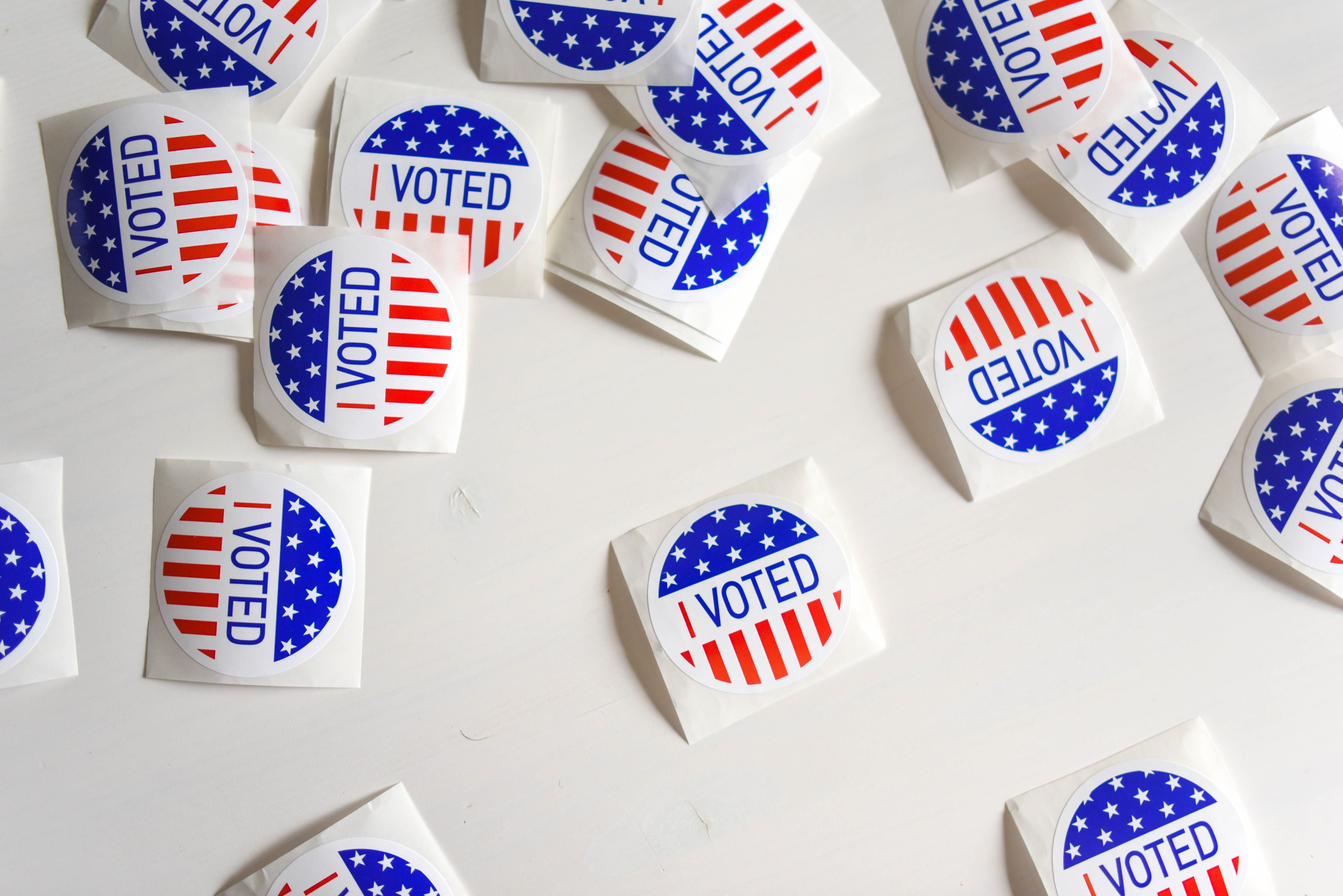
Motivation Example

• Michelle has decided to run for governor of Wisconsin.

• According to previous 30 polls,
  • Michelle’s support is centered round 45%
  • she polled at around 35% in the dreariest days and around 55% in the best days
• With this prior information, we’d like to estimate/update Michelle’s support by conducting a new poll.

Key: Describe prior and data information using probabilistic models.

• The parameter to be estimated is \(\theta\), the Michelle’s support, which is between 0 and 1.

Prior Distribution

• A popular probability distribution for probability is beta distribution, \(\text{beta}(\alpha, \beta)\), where \(\alpha > 0\) and \(\beta > 0\) are shape parameters.

\[\pi(\theta \mid \alpha, \beta) = \frac{\Gamma(\alpha+\beta)}{\Gamma(\alpha)\Gamma(\beta)}\theta^{\alpha - 1}(1-\theta)^{\beta-1}\]

Prior Distribution

• \(\theta \sim \text{beta}(\alpha, \beta)\)

• In the prior model, \(\alpha\) and \(\beta\) are hyperparameters to be chosen to reflect our prior information.

Michelle’s support is centered round 45%, and she polled at around 35% in the dreariest days and around 55% in the best days.

• Choose \(\alpha\) and \(\beta\) so that the prior mean is about 0.45 and the range is from 0.35 to 0.55.

• \(\mathrm{E}(\theta) = \frac{\alpha}{\alpha + \beta}\)

• \(\mathrm{Var}(\theta) = \frac{\alpha\beta}{(\alpha+\beta)^2(\alpha+\beta+1)}\)

Prior Distribution

Likelihood

You plan to conduct a new poll of \(n = 50\) Cheeseheads and record \(Y\), the number that support Michelle.

What distribution can be used for modeling likelihood connecting the data \(y\) and the parameter we are interested, \(\theta\)?

• If voters answer the poll independently, and the probability that any polled voter supports Michelle is \(\theta\), we could consider

\[Y \mid \theta \sim \text{binomial}(n=50, \theta)\]

• The poll result is \(y = 30\), the likelihood is

\[L(\theta \mid y = 30) = {50 \choose 30}\theta^{30}(1-\theta)^{20}, \quad \theta \in (0, 1)\]

Likelihood

Bayesian Model

\[\begin{align}Y \mid \theta &\sim \text{binomial}(n=50, \theta)\\ \theta &\sim \text{beta}(45, 55) \end{align}\]

Goal: Obtain the posterior distribution \(\pi(\theta \mid y)\).

\[ \begin{align} \pi(\theta \mid y) &\propto_{\theta} L(\theta \mid y)\pi(\theta) \\ &= {50 \choose 30}\theta^{30}(1-\theta)^{20} \times \frac{\Gamma(100)}{\Gamma(45)\Gamma(55)}\theta^{44}(1-\theta)^{54}\\ &\propto_{\theta} \theta^{74}(1-\theta)^{74}\\ &= \frac{\Gamma(150)}{\Gamma(75)\Gamma(75)} \theta^{74}(1-\theta)^{74} \\ &= \text{beta}(75, 75)\end{align} \]

using the fact that \(\int_{\mathcal{X}} f(x) dx = 1\) for any pdf \(f(x)\).

Posterior Distribution

Take-home Message

Bayesian/Probabilistic

• The parameter is random
  • The parameter keeps changing.
  • Even the parameter is fixed and constant, the probability distribution associated with it reflects our ignorance, uncertainty, and plausibility of its value, the probability we really want!

Frequentist/Classical

• The parameter is fixed and constant
  • The probability is approximated by relative frequency.
  • The uncertainty is from the randomness of data.

Bayesian Linear Regression*

Normal Data Model

In simple linear regression,

\[Y_i \mid \beta_0, \beta_1, \sigma \stackrel{ind}{\sim} N\left(\mu_i, \sigma^2 \right) \quad \text{with} \quad \mu_i = \beta_0 + \beta_1 X_i\]

This normal data model is our likelihood \(L(\boldsymbol \theta= (\beta_0, \beta_1, \sigma) \mid \mathcal{D} = \{\mathbf{y}, \mathbf{x}\})\), as it evaluates how the data are compatible with different possible values of parameters.

To be a Bayesian, what do we do next?

• Assign priors to the unknown parameters, then do the posterior inference using Bayes’ rule!

• Big question is how?

Prior Models

• There are countless approaches to construct priors for \(\beta_0, \beta_1\), and \(\sigma\).

• For simplicity, assume \(\beta_0, \beta_1\), and \(\sigma\) are independent, \(\pi(\boldsymbol \theta) = \pi(\beta_0, \beta_1, \sigma) = \pi(\beta_0)\pi(\beta_1)\pi(\sigma)\)

• \(\beta_0\) and \(\beta_1\) can technically take any values in the real line.

\[\begin{align} \beta_0 \sim N(m_0, s_0^2) \\ \beta_1 \sim N(m_1, s_1^2) \end{align}\]

• \(\sigma\) must be positive.

\[\begin{align} \sigma \sim \text{Exp}(\lambda) \end{align}\] \(\pi(\sigma) = \lambda e^{-\lambda \sigma}\), \(\lambda > 0\) and \(\mathrm{E}(\sigma) = 1/\lambda\), and \(\mathrm{Var}(\sigma) = 1/\lambda^2\)

https://mc-stan.org/rstanarm/articles/priors.html

Bayesian Simple Linear Regression Model

\[\begin{align} Y_i \mid \beta_0, \beta_1, \sigma &\stackrel{ind}{\sim} N\left(\mu_i, \sigma^2 \right) \quad \text{with} \quad \mu_i = \beta_0 + \beta_1 X_i \\ \beta_0 &\sim N(m_0, s_0^2) \\ \beta_1 &\sim N(m_1, s_1^2) \\ \sigma &\sim \text{Exp}(\lambda) \end{align}\]

Capital Bikeshare bayesrules::bikes Data in Washington, D.C.

Rows: 500
Columns: 2
$ rides     <int> 654, 1229, 1454, 1518, 1362, 891, 1280, 1220, 1137, 1368, 13…
$ temp_feel <dbl> 64.7, 49.0, 51.1, 52.6, 50.8, 46.6, 45.6, 49.2, 46.4, 45.6, …

Tuning Prior Models

• Prior understanding 1:
  • On an average temperature day, say 65 or 70 degrees, there are typically around 5000 riders, though this average could be somewhere between 3000 and 7000.

• The prior information tells us something about \(\beta_0\), but the information has been centered.
  • The centered intercept, \(\beta_{0c}\), reflects the typical ridership at the typical temperature.

\(\beta_{0c} \sim N(5000, 1000^2)\)

Tuning Prior Models

• Prior understanding 2:
  • For every one degree increase in temperature, ridership typically increases by 100 rides, though this average increase could be as low as 20 or as high as 180.

\(\beta_{1} \sim N(100, 40^2)\)

Tuning Prior Models

• Prior understanding 3:
  • At any given temperature, daily ridership will tend to vary with a moderate standard deviation of 1250 rides.

\(\sigma \sim \text{Exp}(0.0008)\) because \(\mathrm{E}(\sigma) = 1/\lambda = 1/0.0008 = 1250\)

Prior Model Simulation

• 100 prior plausible model lines \(\mu_{Y|X} = \beta_0 + \beta_1 X\)

Posterior Inference

• Update our prior understanding of the relationship between ridership and temperature using data information provided by likelihood.

• The joint posterior distribution is

\[\pi(\beta_0, \beta_1, \sigma \mid \mathbf{y}) = \frac{L(\beta_0, \beta_1, \sigma \mid \mathbf{y})\pi(\beta_0, \beta_1, \sigma)}{p(\mathbf{y})}\] where

• \(L(\beta_0, \beta_1, \sigma \mid \mathbf{y}) = p(\mathbf{y}\mid \beta_0, \beta_1, \sigma) = \prod_{i=1}^np(y_i \mid \beta_0, \beta_1, \sigma)\)

• \(\pi(\beta_0, \beta_1, \sigma) = \pi(\beta_0)\pi(\beta_1)\pi(\sigma)\)

• \(p(\mathbf{y}) = \int \int \int \left[\prod_{i=1}^np(y_i \mid \beta_0, \beta_1, \sigma)\right]\pi(\beta_0)\pi(\beta_1)\pi(\sigma) ~ d\beta_0d\beta_1d\sigma\)

• There are lots of ways to generate/approximate the posterior distribution of parameters. One method is Markov chain Monte Carlo (MCMC).

rstanarm::stan_glm()

• rstanarm uses RStan syntax¹ to do Bayesian inference for applied regression models (arm).

bike_model <- rstanarm::stan_glm(rides ~ temp_feel, data = bikes,
                                 family = gaussian,
                                 prior_intercept = normal(5000, 1000),
                                 prior = normal(100, 40), 
                                 prior_aux = exponential(0.0008),
                                 chains = 4, iter = 5000*2, seed = 2025)

• Generate 4 Monte Carlo chains (chains = 4), each having 10000 iterations (iter = 5000*2).

• Each iteration draw a posterior sample of the \(\beta_0\), \(\beta_1\), and \(\sigma\).

• After tossing out the first half of Markov chain values from the warm-up or burn-in phase, stan_glm() simulation produces four parallel chains of length 5000 for each model parameter:

\(\{ \beta_0^{(1)}, \beta_0^{(2)}, \dots, \beta_0^{(5000)} \}\), \(\{ \beta_1^{(1)}, \beta_1^{(2)}, \dots, \beta_1^{(5000)} \}\), \(\{ \sigma^{(1)}, \sigma^{(2)}, \dots, \sigma^{(5000)} \}\)

1. RStan is the R interface to Stan.

Convergence Diagnostics

# Trace plots of parallel chains
bayesplot::mcmc_trace(bike_model, size = 0.1)

Convergence Diagnostics

Source: https://blog.stata.com/2016/11/15/introduction-to-bayesian-statistics-part-2-mcmc-and-the-metropolis-hastings-algorithm/

Convergence Diagnostics

Convergence Diagnostics

# Density plots of parallel chains
bayesplot::mcmc_dens_overlay(bike_model)

• quantifies the number of independent samples it would take to produce an equivalently accurate posterior approximation.
• we observe that these four chains produce nearly indistinguishable posterior approximations. This provides evidence that our simulation is stable and sufficiently long – running the chains for more iterations likely wouldn’t produce drastically different or improved posterior approximations.

Convergence Diagnostics

# Effective sample size ratio
bayesplot::neff_ratio(bike_model)

(Intercept)   temp_feel       sigma 
      0.995       0.992       0.950 

# Rhat
bayesplot::rhat(bike_model)

(Intercept)   temp_feel       sigma 
          1           1           1 

• Both effective sample size and R-hat are close to 1, indicating that the chains are stable, mixing quickly, and behaving much like an independent sample.

• There’s no magic rule for interpreting this ratio, and it should be utilized alongside other diagnostics such as the trace plot. That said, we might be suspicious of a Markov chain for which the effective sample size ratio is less than 0.1, i.e., the effective sample size is less than 10% of the actual sample size.
• an R-hat ratio greater than 1.05 raises some red flags about the stability of the simulation.

Convergence Issues

• Highly Autocorrelated Chain: Effective size is small, not many independent samples that are representative of the true posterior distribution.
  • Run longer and thinning the chain

• Slow Convergence: Need wait longer to have the chain reached a stable mixing zone that are representative of the true posterior distribution.
  • Set a longer burn-in or warm-up period

Interpreting the Posterior

# Posterior summary statistics
tidy(bike_model, effects = c("fixed", "aux"),
     conf.int = TRUE, conf.level = 0.80)

# A tibble: 4 × 5
  term        estimate std.error conf.low conf.high
  <chr>          <dbl>     <dbl>    <dbl>     <dbl>
1 (Intercept)  -2191.     355.    -2653.    -1735. 
2 temp_feel       82.1      5.07     75.7      88.7
3 sigma         1282.      41.1    1231.     1336. 
4 mean_PPD      3487.      80.3    3385.     3590. 

• The posterior relationship is

\[-2196 + 82.2 X\]

• The 80% credible interval for \(\beta_1\) is \((75.7, 88.5)\).

• Given the data, the probability that \(\beta_1\) is between 75.7 and 88.5 is 80%., i.e., \(P(\beta_1 \in(75.7, 88.5) \mid \mathbf{y}, \mathbf{x}) = 80\%\).

Posterior Samples

# Store the 4 chains for each parameter in 1 data frame
bike_model_df <- as.data.frame(bike_model)
nrow(bike_model_df)

[1] 20000

head(bike_model_df)

  (Intercept) temp_feel sigma
1       -2318      83.0  1304
2       -2107      81.9  1261
3       -2460      85.9  1246
4       -2419      84.7  1394
5       -2067      79.5  1202
6       -1806      75.6  1224

How to obtain \(P(\beta_1 > 0 \mid \mathbf{y}, \mathbf{x})\)?

\(P(\beta_1 > 0 \mid \mathbf{y}, \mathbf{x}) \approx \frac{1}{20000}\sum_{t=1}^{20000} \mathbf{1}\left(\beta_1^{(t)} > 0\right)\)

sum(bike_model_df$temp_feel > 0) / nrow(bike_model_df)

[1] 1

Posterior Regression Lines

Posterior Predictive Draws

For each posterior draw \(\{\beta_0^{(t)}, \beta_1^{(t)}, \sigma^{(t)} \}_{t = 1}^{20000}\), we have the posterior predictive distribution \[Y_i^{(t)} \sim N\left(\beta_0^{(t)} + \beta_1^{(t)}X_i, \, (\sigma^{(t)})^2\right)\]

Bayesian Interpretation for Ridge and Lasso

• Lasso and Ridge regression can be interpreted as a Bayesian regression model.

• The same data-level likelihood \[Y_i \mid \boldsymbol \beta, \sigma \stackrel{ind}{\sim} N\left(\mu_i, \sigma^2 \right) \quad \text{with} \quad \mu_i = \mathbf{x}_i'\boldsymbol \beta\]

• We use prior distributions to regularize how parameters behave.

• The two methods can assign the same prior distributions to \(\beta_0\) and \(\sigma\), but they use different priors on \(\{\beta_j\}_{j = 1}^p\).¹

  • Lasso: \(\beta_j \stackrel{iid}{\sim} \text{Laplace}\left(0, \tau(\lambda)\right)\)

  • Ridge: \(\beta_j \stackrel{iid}{\sim} N\left(0, \tau(\lambda)\right)\)

1. Remember we usually standardize coefficients before implementing Ridge and Lasso.

Ridge and Lasso Priors

Lasso

\[\beta_j \stackrel{iid}{\sim} \text{Laplace}\left(0, \tau(\lambda)\right)\]

Lasso solution is the posterior mode of \(\boldsymbol \beta\)

\[\boldsymbol \beta^{(l)} = \mathop{\mathrm{arg\,max}}_{\boldsymbol \beta} \,\,\, \pi(\boldsymbol \beta\mid \mathbf{y}, \mathbf{x})\]

Ridge

\[\beta_j \stackrel{iid}{\sim} N\left(0, \tau(\lambda)\right)\]

Ridge solution is the posterior mode/mean of \(\boldsymbol \beta\)

\[\boldsymbol \beta^{(r)} = \mathop{\mathrm{arg\,max}}_{\boldsymbol \beta} \,\, \, \pi(\boldsymbol \beta\mid \mathbf{y}, \mathbf{x})\]

Resources

• Bayes Rules! An Introduction to Applied Bayesian Modeling

• Statistical Rethinking

• A Student’s Guide to Bayesian Statistics

• Bayesian Data Analysis