Logistic Regression

MSSC 6250 Statistical Machine Learning

Dr. Cheng-Han Yu
Department of Mathematical and Statistical Sciences
Marquette University

Binary Logistic Regression

Non-Gaussian and Non-continuous Response

• In many applications, the response or error term are nonnormal.

  • Binary response: how an online banking system determine whether or not a transaction is fraudulent based on the user’s IP address.
  • Count response: how weather conditions affect the number of users of a bike sharing program during a particular hour of the day.

• Besides normal, the response in a generalized linear model (GLM) can be Bernoulli, binomial, Poisson, etc.

• There is no assumption that \(\mathrm{Var}(y_i)\) is homogeneous: Both \(E(y_i)\) and \(\mathrm{Var}(y_i)\) may vary with the regressors from data point to data point.

• Ordinary least squares does not apply when the response is not normal.

Classification

• Linear regression assumes that the response \(Y\) is numerical.
• In many situations, \(Y\) is categorical.

• A process of predicting categorical response is known as classification.

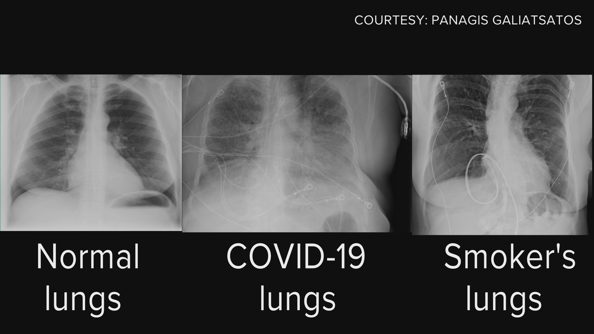
Normal vs. COVID vs. Smoking

fake news vs. true news

Regression Function \(f(x)\) vs. Classifier \(C(x)\)

https://daviddalpiaz.github.io/r4sl/classification-overview.html

Soft and Hard Classifiers

Two popular approaches when modeling binary data

• Soft classifiers
  • Estimate the conditional probabilities \(Pr(Y = k \mid {\bf X})\) for each category \(k\).
  • Use \(\mathbf{1}\{Pr(Y \mid {\bf X}) > c \}\) for classification, where \(c \in(0, 1)\) is a threshold or cutoff.
  • e.g. logistic regression

• Hard classifiers
  • Directly estimate the classification decision boundary
  • e.g. support vector machines

Classification Example

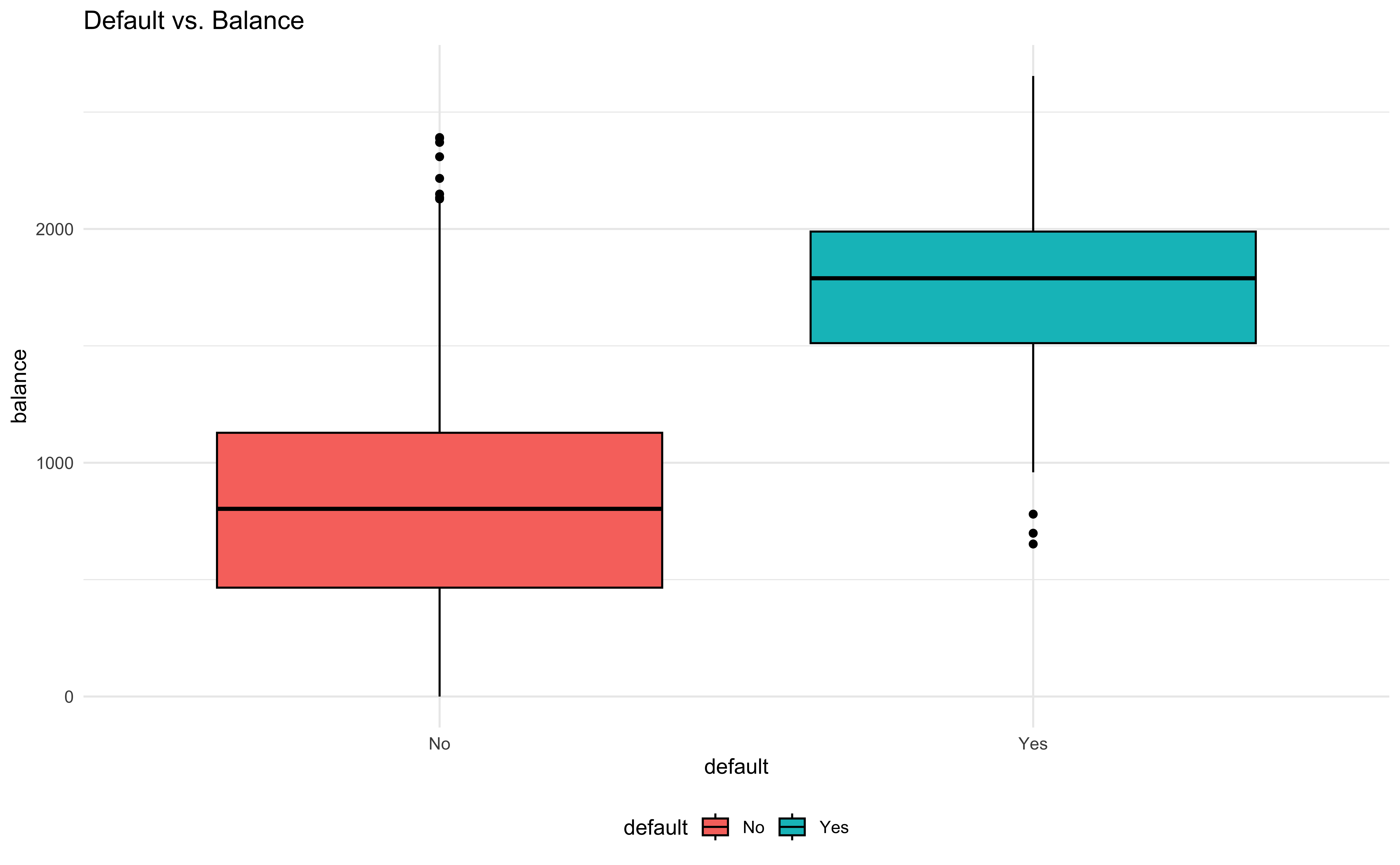
Given the training data \(\{(x_i, y_i)\}_{i=1}^n\), we build a classifier to predict whether people will default on their credit card payment \((Y)\) yes or no, based on monthly credit card balance \((X)\).

Why Not Linear Regression

\[Y =\begin{cases} 0 & \quad \text{if not default}\\ 1 & \quad \text{if default} \end{cases}\]

• \(Y = \beta_0 + \beta_1X + \epsilon\), \(\, X =\) credit card balance

What are potential issues with this dummy variable approach?

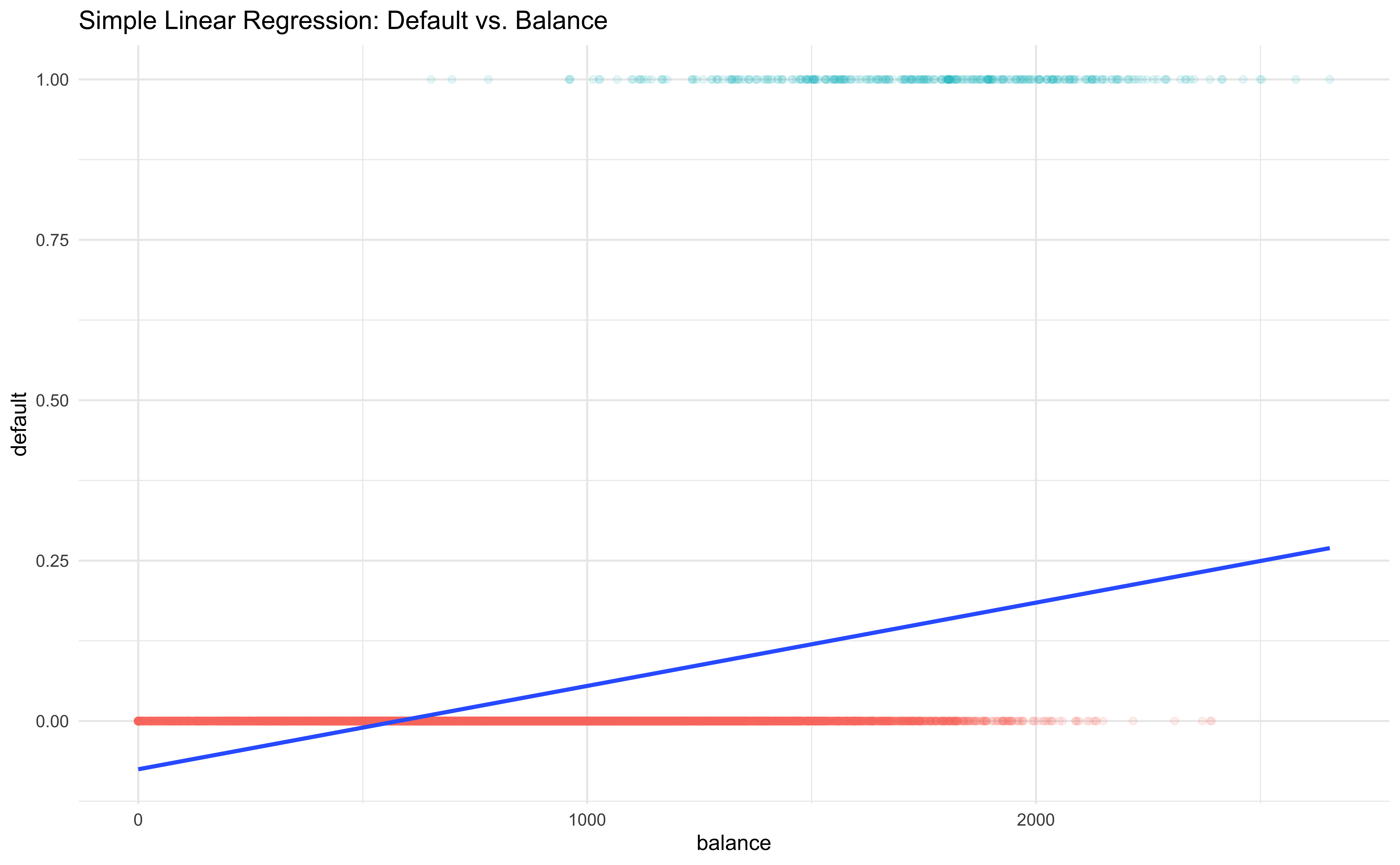
• \(\hat{Y} = b_0 + b_1X\) estimates \(P(Y = 1 \mid X) = P(default = yes \mid balance)\).

• However,

Why Not Linear Regression?

• Probability estimates can be outside \([0, 1]\).

Why Not Linear Regression?

• Linear regression generally cannot handle more than two categories.

\[Y =\begin{cases} 1 & \quad \text{stroke}\\ 2 & \quad \text{drug overdose} \\ 3 & \quad \text{epileptic seisure} \end{cases}\]

• The coding

  • suggests an ordering epileptic seisure \(>\) drug overdose \(>\) stroke
  • implies that stroke \(-\) drug overdose \(=\) drug overdose \(-\) epileptic seizure.

Binary Logistic Regression

• First predict the probability of each category of \(Y\)
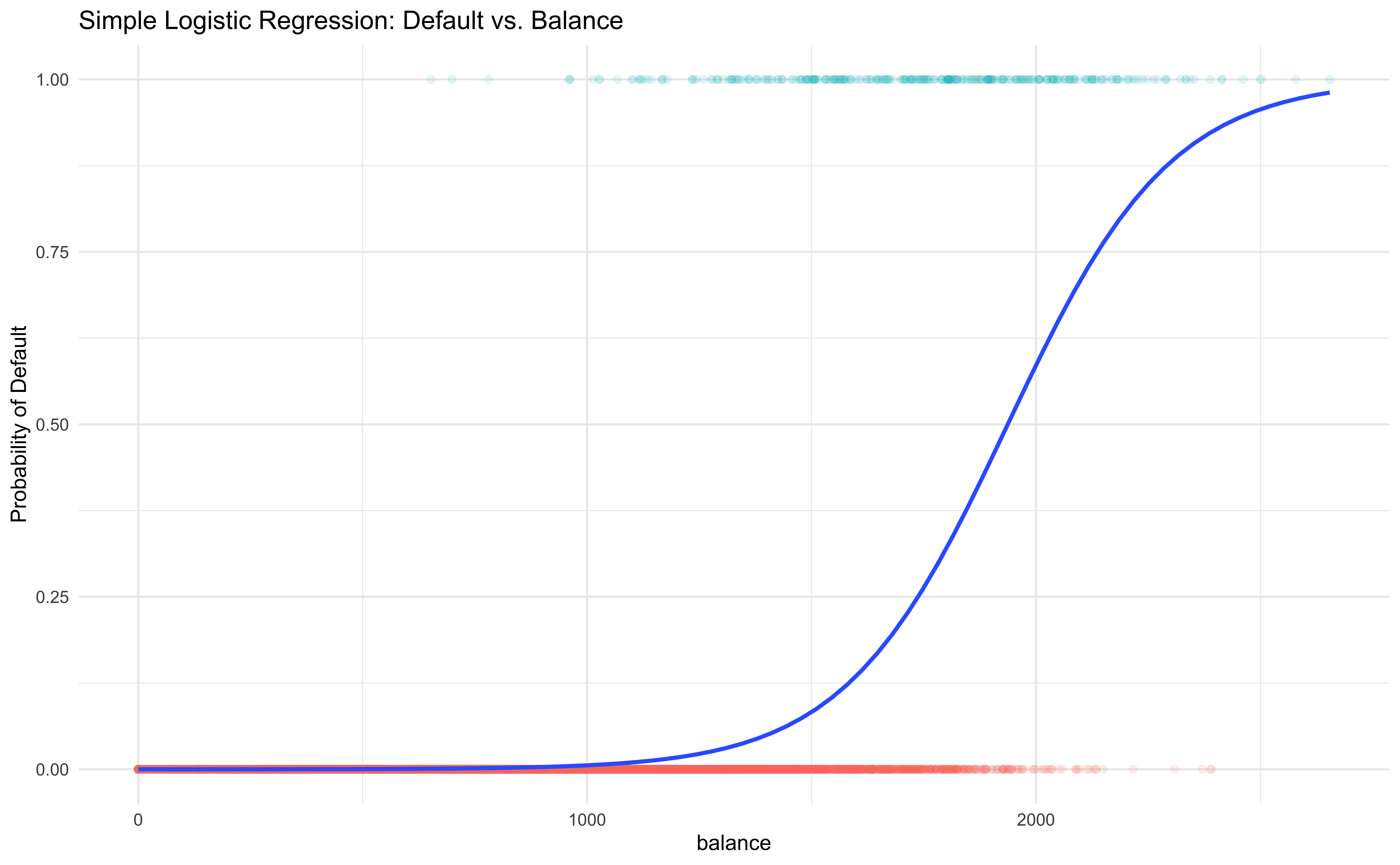
• Predict probability of default using a S-shaped curve.

Framing the Problem: Binary Responses

We use normal distribution for numerical \(y\). What distribution we can use for binary \(y\) that takes value 0 or 1?

• Each outcome default \((y = 1)\) and not default \((y = 0)\) is a Bernoulli variable. But,

• The probability of “success” \(\pi\) is not constant but varies with predictor values!

\[ y_i \mid x_i \stackrel{indep}{\sim} \text{Bernoulli}(\pi_i = \pi(x_i)) = \text{binomial}(m=1,\pi = \pi_i) \]

• \(X =\) balance. \(x_1 = 2000\) has a larger \(\pi_1 = \pi(2000)\) than \(\pi_2 = \pi(500)\) with \(x_2 = 500\)
• Credit cards with a higher balance are more likely to be defaulted.

In the credit card example, - do we have exactly two outcomes? - do we have constant probability? \(P(y_1 = 1) = P(y_2 = 1) = \cdots = P(y_n = 1) = \pi?\) Exactly the same idea as linear regression, where the the mean response is not constant but varies with the value of predictors, \(E(y_i) = \beta_0+\beta_1x_i\).

Logistic Function

Instead of predicting \(y_i\) directly, we use the predictors to model its probability of success, \(\pi_i\).

But how?

• Transform \(\pi \in (0, 1)\) into a variable \(\eta \in (-\infty, \infty)\). Then construct a linear predictor on \(\eta\): \(\eta_i = \mathbf{x}_i'\boldsymbol \beta\)

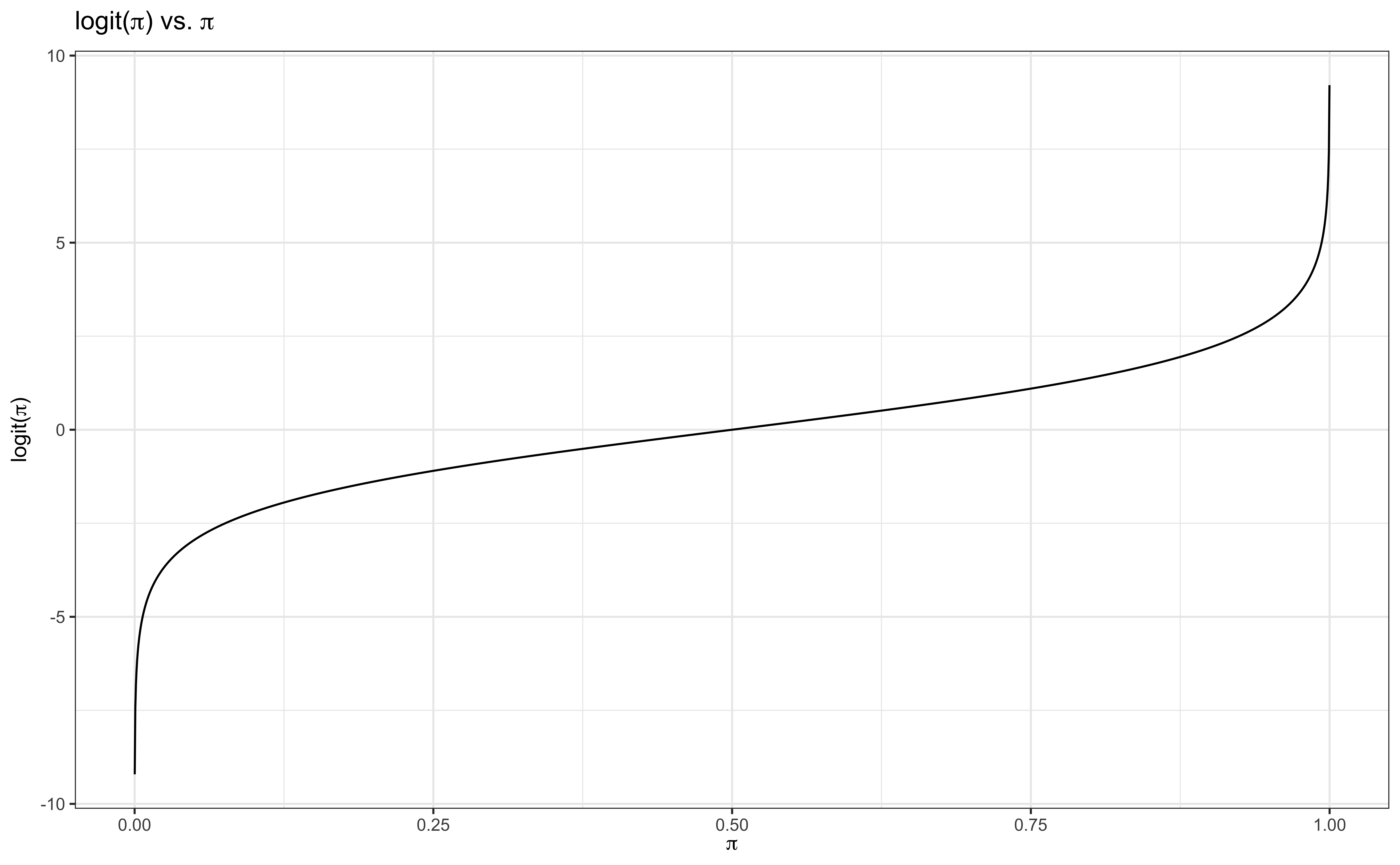
• Logit function: For \(0 < \pi < 1\)

\[\eta = \text{logit}(\pi) = \ln\left(\frac{\pi}{1-\pi}\right)\]

Logit function \(\eta = \text{logit}(\pi) = \ln\left(\frac{\pi}{1-\pi}\right)\)

Logistic Function

• The logit function \(\eta = \text{logit}(\pi) = \ln\left(\frac{\pi}{1-\pi}\right)\) takes a value \(\pi \in (0, 1)\) and maps it to a value \(\eta \in (-\infty, \infty)\).
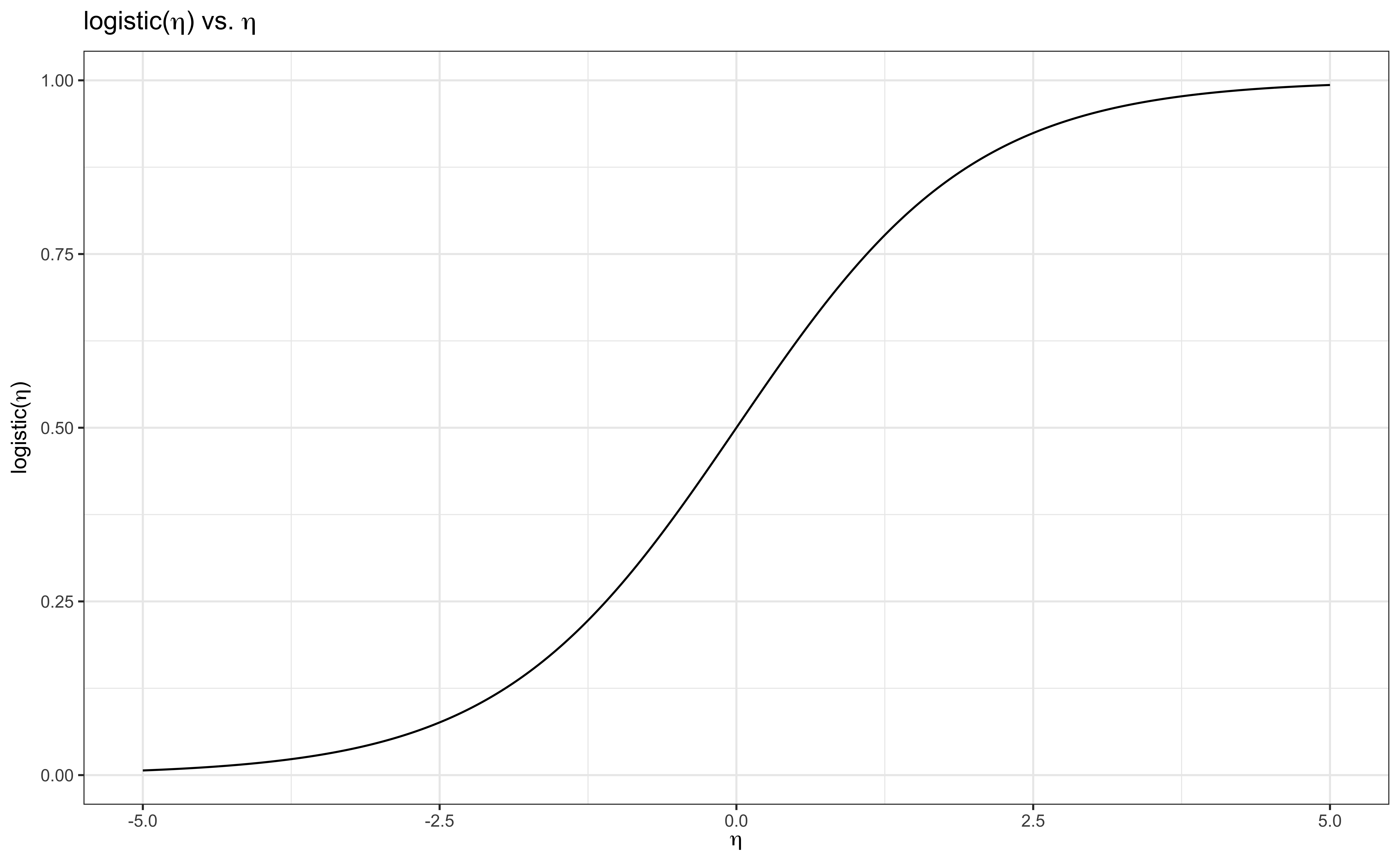
• Logistic function: \[\pi = \text{logistic}(\eta) = \frac{1}{1+\exp(-\eta)} \in (0, 1)\]
• The logistic (sigmoid) function takes a value \(\eta \in (-\infty, \infty)\) and maps it to a value \(\pi \in (0, 1)\).

• Once \(\eta\) is estimated by the linear regression, we use the logistic function to transform \(\eta\) back to the probability.

\[\pi = \text{logistic}(\eta) = \frac{\exp(\eta)}{1+\exp(\eta)} = \frac{1}{1+\exp(-\eta)} \in (0, 1)\]

Logistic (Sigmoid) Function \(\pi = \text{logistic}(\eta) = \frac{1}{1+\exp(-\eta)}\)

Logistic Regression Model

For \(i = 1, \dots, n\) and with \(p\) predictors: \[Y_i \mid \pi_i({\bf x}_i) \stackrel{indep}{\sim} \text{Bernoulli}(\pi_i), \quad {\bf x}_i' = (x_{i1}, \dots, x_{ip})\] \[\text{logit}(\pi_i) = \ln \left( \frac{\pi_i}{1 - \pi_i} \right) = \eta_i = \beta_0+\beta_1 x_{i1} + \cdots + \beta_p x_{ip} = {\bf x}_i'\boldsymbol \beta\]

• The \(\eta_i = \text{logit}(\pi_i)\) is a link function that links the linear predictor and the mean of \(Y_i\).

\[\small E(Y_i) = \pi_i = \frac{1}{1 + \exp(-{\bf x}_i'\boldsymbol \beta)}\] \[\small \hat{\pi}_i = \frac{1}{1 + \exp(-{\bf x}_i'\hat{\boldsymbol \beta} )}\]

Default Data in ISLR2

data("Default"); head(Default, 10)

   default student balance income
1       No      No     730  44362
2       No     Yes     817  12106
3       No      No    1074  31767
4       No      No     529  35704
5       No      No     786  38463
6       No     Yes     920   7492
7       No      No     826  24905
8       No     Yes     809  17600
9       No      No    1161  37469
10      No      No       0  29275

str(Default)

'data.frame':   10000 obs. of  4 variables:
 $ default: Factor w/ 2 levels "No","Yes": 1 1 1 1 1 1 1 1 1 1 ...
 $ student: Factor w/ 2 levels "No","Yes": 1 2 1 1 1 2 1 2 1 1 ...
 $ balance: num  730 817 1074 529 786 ...
 $ income : num  44362 12106 31767 35704 38463 ...

Fitting ¹

logit_fit <- glm(default ~ balance, data = Default, 
                 family = binomial)
coef(summary(logit_fit))

            Estimate Std. Error z value Pr(>|z|)
(Intercept) -10.6513    0.36116     -29 3.6e-191
balance       0.0055    0.00022      25 2.0e-137

\(\hat{\eta} = \text{logit}(\hat{\pi}) = \ln \left( \frac{\hat{\pi}}{1 - \hat{\pi}}\right) = -10.65 + 0.0055 \times \text{balance}\)

1. In Python, use statsmodels.formula.api.logit or sklearn.linear_model.LogisticRegression

Interpretation of Coefficients

The ratio \(\frac{\pi}{1-\pi} \in (0, \infty)\) is called the odds of some event.

• Example: If 1 in 5 people will default, the odds is 1/4 since \(\pi = 0.2\) implies an odds of \(0.2/(1−0.2) = 1/4\).

\[\ln \left( \frac{\pi(x)}{1 - \pi(x)} \right)= \beta_0 + \beta_1x\]

• Increasing \(x\) by one unit
  • changes the log-odds by \(\beta_1\)
  • multiplies the odds by \(e^{\beta_1}\)

• \(\beta_1\) does not correspond to the change in \(\pi(x)\) associated with a one-unit increase in \(x\).
• \(\beta_1\) is the change in log odds associated with one-unit increase in \(x\).

Interpretation of Coefficients

            Estimate Std. Error z value Pr(>|z|)
(Intercept)  -10.651       0.36     -29        0
balance        0.005       0.00      25        0

• \(\hat{\eta} = \text{logit}(\hat{\pi}) = \ln \left( \frac{\hat{\pi}}{1 - \hat{\pi}}\right) = -10.65 + 0.0055 \times \text{balance}\)

• \(\hat{\eta}(x) = \hat{\beta}_0 + \hat{\beta}_1x\)
• \(\hat{\eta}(x+1) = \hat{\beta}_0 + \hat{\beta}_1(x+1)\)
• \(\hat{\eta}(x+1) - \hat{\eta}(x) = \hat{\beta}_1 = \ln(\text{odds}_{x+1}) - \ln(\text{odds}_{x})\)
• One-unit increase in balance increases the log odds of default by 0.005 units.

• The odds ratio, \(\widehat{OR} = \frac{\text{odds}_{x+1}}{\text{odds}_{x}} = e^{\hat{\beta}_1} = e^{0.0055} = 1.005515\).
• The odds of default increases by 0.5% with additional one unit of credit card balance.

Pr(default) When Balance is 2000

\[\log\left(\frac{\hat{\pi}}{1-\hat{\pi}}\right) = -10.65+0.0055\times 2000\]

\[ \hat{\pi} = \frac{1}{1+\exp(-(-10.65+0.0055 \times 2000)} = 0.586\]

pi_hat <- predict(logit_fit, type = "response")
eta_hat <- predict(logit_fit, type = "link")  ## default gives us b0 + b1*x
predict(logit_fit, newdata = data.frame(balance = 2000), type = "response")

   1 
0.59 

Probability Curve

What is the probability of default when the balance is 500? What about balance 2500?

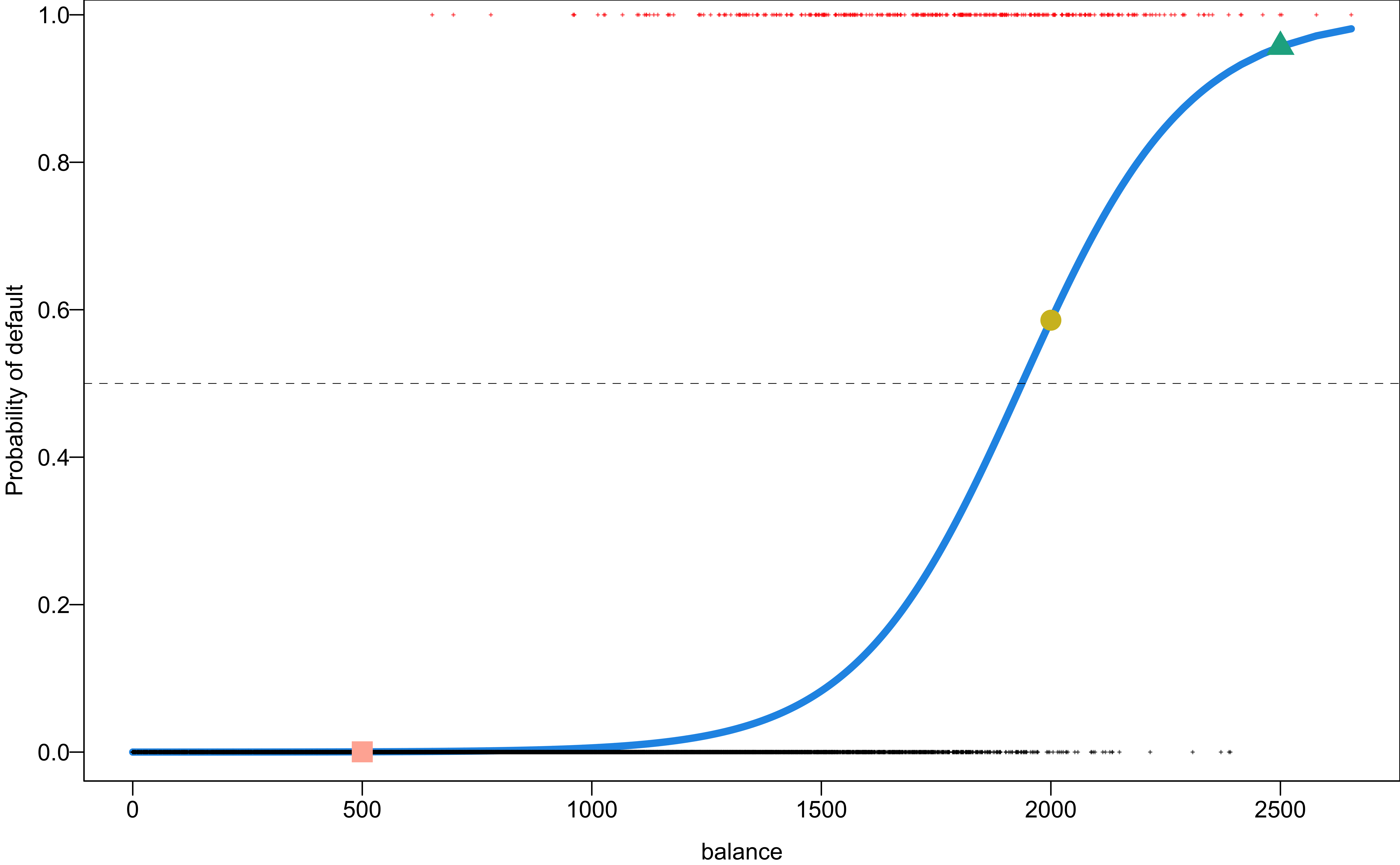
• 500 balance: Pr(default) = 0
• 2000 balance: Pr(default) = 0.59
• 2500 balance: Pr(default) = 0.96

Maximum Likelihood Estimation

• glm() uses maximum likelihood to estimate the parameters \(\boldsymbol \beta\).

The log-likelihood is given by

\[\ell(\boldsymbol \beta) = \sum_{i=1}^n \log \, p(y_i \mid x_i, \boldsymbol \beta).\]

Using Bernoulli probabilities, we have

\[\begin{align} \ell(\boldsymbol \beta) =& \sum_{i=1}^n \log \left\{ \pi(\mathbf{x}_i)^{y_i} [1-\pi(\mathbf{x}_i)]^{1-y_i} \right\}\\ =& \sum_{i=1}^n y_i \log \frac{\pi(\mathbf{x}_i)}{1-\pi(\mathbf{x}_i)} + \log [1-\pi(\mathbf{x}_i)] \\ =& \sum_{i=1}^n y_i \mathbf{x}_i' \boldsymbol \beta- \log [ 1 + \exp(\mathbf{x}_i' \boldsymbol \beta)] \end{align}\]

Maximum Likelihood Estimation

• We can use Newton’s method that needs the gradient and Hessian matrix.

\[\boldsymbol \beta^{\text{new}} = \boldsymbol \beta^{\text{old}} - \left[ \frac{\partial ^2 \ell(\boldsymbol \beta)}{\partial \boldsymbol \beta\partial \boldsymbol \beta'}\right] ^{-1}\frac{\partial \ell(\boldsymbol \beta)}{\partial \boldsymbol \beta}\]

• Simply use optim()

x <- as.matrix(cbind("intercept" = 1, Default$balance))
y <- as.matrix(as.numeric(Default$default) - 1)
beta <- rep(0, ncol(x))  ## start with 0

optim(beta, fn = my_loglik, gr = my_gradient, method = "BFGS", 
      x = x, y = y, 
      control = list("fnscale" = -1))$par # "fnscale" = -1 for maximization

[1] -10.6454   0.0055

Evaluation¹

• Confusion Matrix

	True 0	True 1
Predict 0	True Negative (TN)	False Negative (FN)
Predict 1	False Positive (FP)	True Positive (TP)

• Sensitivity (True Positive Rate) \(= P( \text{predict 1} \mid \text{true 1}) = \frac{TP}{TP+FN}\)

• Specificity (True Negative Rate) \(= P( \text{predict 0} \mid \text{true 0}) = \frac{TN}{FP+TN}\)

• Accuracy \(= \frac{TP + TN}{TP+FN+FP+TN} = \frac{1}{m}\sum_{j=1}^mI(y_j = \hat{y}_j)\), where \(y_j\)s are true test labels and \(\hat{y}_j\)s are their corresponding predicted label.

A good classifier can be the one which the test accuracy rate is highest, or test error rate \(\frac{1}{m}\sum_{j=1}^mI(y_j \ne \hat{y}_j)\) is smallest.

1. More on Wiki page.

Confusion Matrix ¹

pred_prob <- predict(logit_fit, type = "response")
table(pred_prob > 0.5, Default$default)

       
          No  Yes
  FALSE 9625  233
  TRUE    42  100

• Packages:
  • caret (Classification And REgression Training)
  • yardstick of tidymodels

caret::confusionMatrix()
yardstick::conf_mat()

1. For simplicity we use training set for demo. In real applications, we care about the classification result of the test set.

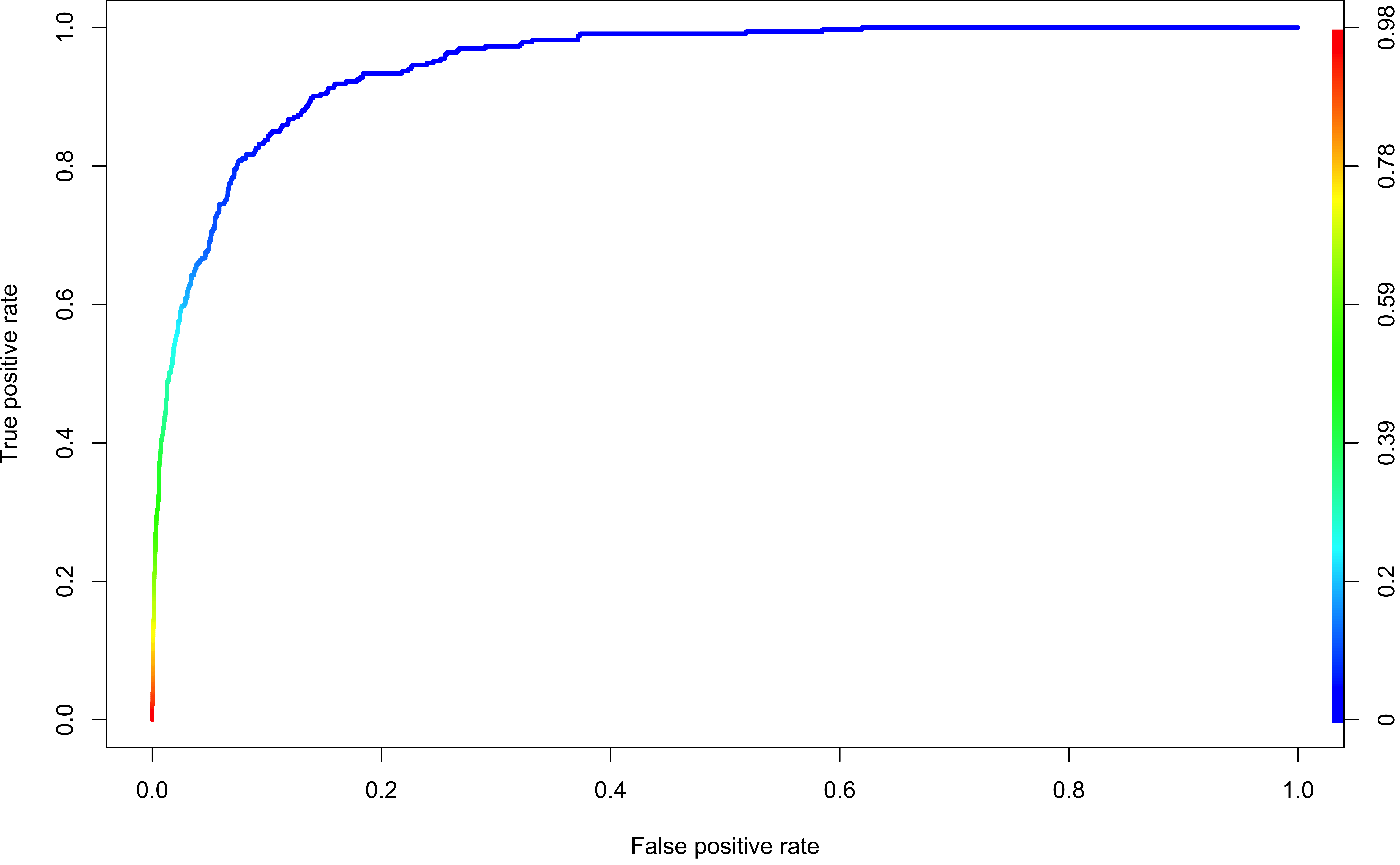
Receiver Operating Characteristic (ROC) Curve

• The ROC curve plots True Positive Rate (Sensitivity) vs. False Positive Rate (1 - Specificity)

• ROC Plot
• Code

library(ROCR)
# create an object of class prediction 
pred <- ROCR::prediction(
    predictions = pred_prob, 
    labels = Default$default)
# calculates the ROC curve
roc <- ROCR::performance(
    prediction.obj = pred, 
    measure = "tpr",
    x.measure = "fpr")
plot(roc, colorize = TRUE, lwd = 3)

• Packages: ROCR, pROC, yardstick::roc_curve()

Area Under Curve (AUC)

Find the area under the curve:

## object of class 'performance'
auc <- ROCR::performance(
    prediction.obj = pred, 
    measure = "auc")
auc@y.values

[[1]]
[1] 0.95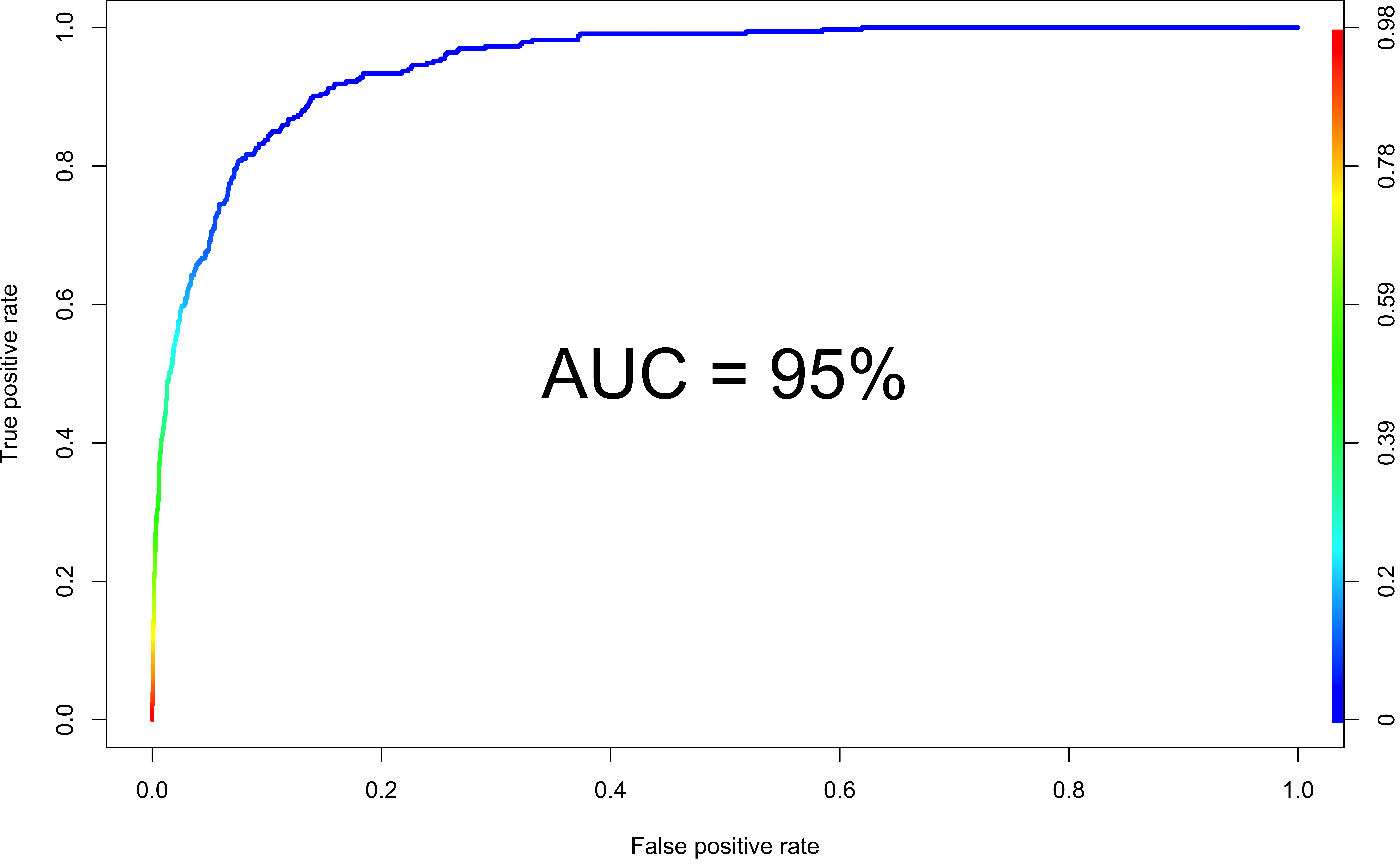

Precision-recall curve

Threshold 0.5 Issue

• Threshold 0.5 may be inappropriate if
  • imbalanced data or skewed class distribution in training
  • the cost of one type of misclassification is more important than another.

• 0.5 threshold may misclassify too many minority class samples. Using smaller threshold Example: If only 1% of the data is fraud, a model predicting “no fraud” for everything would still achieve 99% accuracy, but it fails at detecting fraud.
• If false positive is more costly (Marking a real email as spam (False Positive) can be frustrating), want to be more conservative, so use larger threshold.
• If false negative is more costly (Medical Diagnosis: Missing cancer (False Negative) is much worse), want to be more aggressive, so use smaller threshold.

Optimal Threshold

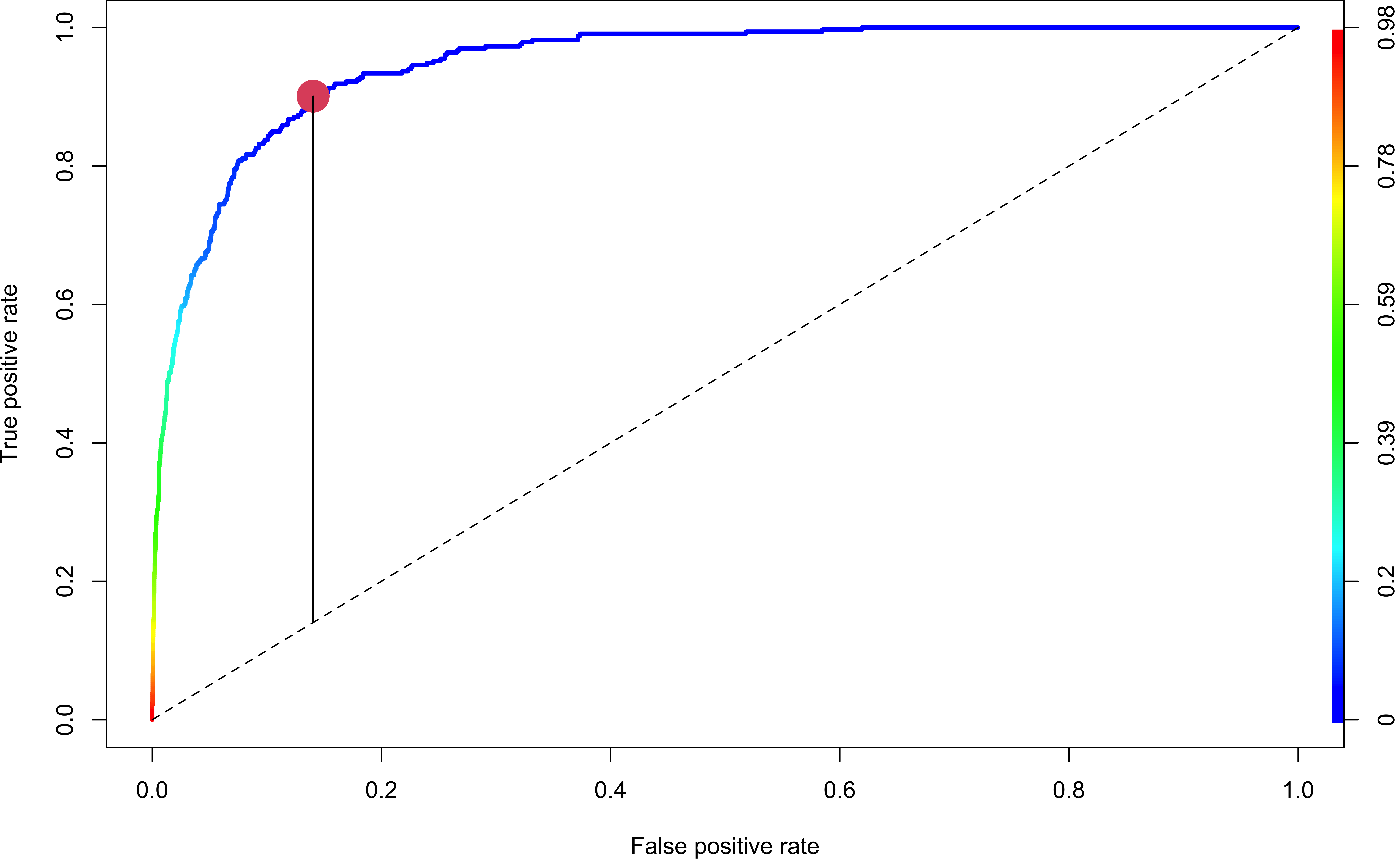
From the training set, choose the cut-off that maximizes

• G-Mean \(= \sqrt{\text{TPR} * \text{TNR}}\) (geometric mean of TPR and TNR)

• Youden’s J index \(= \text{TPR} + \text{TNR} - 1\) (the distance to the 45 degree identity line)

or that minimizes

• D-optimal Threshold \(= \sqrt{(1 - \text{TPR})^2 + (1 - \text{TNR})^2}\) (the distance to the optimal point)

G-mean used When dealing with imbalanced datasets (rare events).

Youden’s J Index used when Equal importance of positives & negatives.

D-optimal Threshold Does not assume class balance, unlike some other metrics. When minimizing both false positives and false negatives.

Optimal Threshold

With Youden’s J index, the optimal threshold is \(3.18\%\).

• The predicted probabilities are not calibrated, e.g. those predicted by an SVM or decision tree.
• The metric used to train the model is different from the metric used to evaluate a final model.
• The class distribution is severely skewed.
• The cost of one type of misclassification is more important than another type of misclassification.
• Learning from Imbalanced Data Sets 1st ed. 2018 Edition
• https://machinelearningmastery.com/threshold-moving-for-imbalanced-classification/ The index is represented graphically as the height above the chance line, and it is also equivalent to the area under the curve subtended by a single operating point. https://web.expasy.org/pROC/files/pROC_1.7.2_R_manual.pdf

Multinomial Logistic Regression

Multinomial Logistic Regression

• When classifying \(K > 2\) categories, we can consider multinomial logistic regression¹.

• The response should be nominal. If \(Y_i\) is ordinal, we should consider the ordinal regression.

1. Sometimes it is known as multiclass logistic regression.

Multinomial Link

• First select a single class to serve as the baseline, the \(K\)th class for example.¹

For \(k = 1, 2, \dots, K-1,\)

\[Pr(Y = k \mid {\bf x}) = \dfrac{e^{\beta_{k0}+\beta_{k1}x_1 + \cdots + \beta_{kp}x_p}}{ \sum_{l=1}^{K}e^{\beta_{l0}+\beta_{l1}x_1 + \cdots + \beta_{lp}x_p}},\] and \[Pr(Y = K \mid {\bf x}) = \dfrac{1}{ \sum_{l=1}^{K}e^{\beta_{l0}+\beta_{l1}x_1 + \cdots + \beta_{lp}x_p}}.\]

For \(k = 1, \dots, K-1\), \[\log\left( \frac{Pr(Y = k \mid \mathbf{x})}{Pr(Y = K \mid \mathbf{x})} \right) = \beta_{k0}+\beta_{k1}x_1 + \cdots + \beta_{kp}x_p.\]

1. The coefficient estimates will differ if a different baseline is used. But the fitted values, predictions, log odds between any pair of classes remain the same.

Multinomial Link

• First select a single class to serve as the baseline, the \(K\)th class for example.¹

• \(\pi_{ik} = Pr(Y_i = k \mid {\bf x}_i)\): the probability that the \(i\)-th response falls in the \(k\)-th category.

• \(\sum_{k = 1}^K \pi_{ik} = 1\) for each observation \(i\).

• For \(k = 1, \dots, K-1\), the link \(\eta_{ik} = \log\left( \frac{\pi_{ik}}{\pi_{iK}}\right) = \beta_{k0}+\beta_{k1}x_1 + \cdots + \beta_{kp}x_p = {\bf x}_i'\boldsymbol \beta_k\), where \(\boldsymbol \beta_k = (\beta_{k0}, \beta_{k1}, \dots, \beta_{kp})'\)

What is the value of \(\eta_{iK}\)?

For \(k = 1, \dots, K\),

\[\pi_{ik} = \dfrac{e^{\eta_{ik}}}{\sum_{l=1}^{K}e^{\eta_{il}}}; \left(\pi_{iK} = \dfrac{1}{\sum_{l=1}^{K}e^{\eta_{il}}} \right)\]

1. The coefficient estimates will differ if a different baseline is used. But the fitted values, predictions, log odds between any pair of classes remain the same.

Multinomial Data

Rows: 200
Columns: 3
$ prog  <fct> vocation, general, vocation, vocation, vocation, general, vocati…
$ ses   <fct> low, middle, high, low, middle, high, middle, middle, middle, mi…
$ write <dbl> 35, 33, 39, 37, 31, 36, 36, 31, 41, 37, 44, 33, 31, 44, 35, 44, …

• Response:
  • prog (program type: general, academic, vocation)
• Predictors:
  • ses (social economic status: low, middle, high)
  • write (writing score)

Entering high school students make program choices among general program, vocational program and academic program. Their choice might be modeled using their writing score and their social economic status.

Multinomial Logit - Variable Association

Program type is affected by social economic status

        prog
ses      general academic vocation
  low         16       19       12
  middle      20       44       31
  high         9       42        7

and writing score

          M  SD
general  51 9.4
academic 56 7.9
vocation 47 9.3

The level (coding order) of prog is

[1] "general"  "academic" "vocation"

Multinomial Logit - Setting Baseline

multino_data$prog2 <- relevel(multino_data$prog, ref = "academic")
levels(multino_data$prog2)

[1] "academic" "general"  "vocation"

• academic = 1 (baseline), general = 2, vocation = 3
• For ses, low = 1 (baseline), middle = 2, high = 3

\[\log \left( \frac{Pr(prog = general)}{Pr(prog = academic)}\right) = b_{10} + b_{11}I(ses = 2) + b_{12}I(ses = 3) + b_{13}write\]

\[\log \left( \frac{Pr(prog = vocation)}{Pr(prog = academic)}\right) = b_{20} + b_{21}I(ses = 2) + b_{22}I(ses = 3) + b_{23}write\]

All others held constant,

• \(b_{13}\): the amount changed in the log odds of being in general vs. academic program as write increases one unit.

• \(b_{21}\) the amount changed in the log odds of being in vocation vs. academic program if moving from ses = "low" to ses = "middle".

set “academic” as the baseline category factor(multino_data$prog, levels = c(“general”, “vocation”, “academic”) b13 A one-unit increase in the variable write is associated with the decrease in the log odds of being in general program vs. academic program in the amount of .058 . b23 A one-unit increase in the variable write is associated with the decrease in the log odds of being in vocation program vs. academic program. in the amount of .1136 . b12 The log odds of being in general program vs. in academic program will decrease by 1.163 if moving from ses=“low” to ses=“high”. b11 The log odds of being in general program vs. in academic program will decrease by 0.533 if moving from ses=“low”to ses=“middle”, although this coefficient is not significant. b22 The log odds of being in vocation program vs. in academic program will decrease by 0.983 if moving from ses=“low” to ses=“high”. b21 The log odds of being in vocation program vs. in academic program will increase by 0.291 if moving from ses=“low” to ses=“middle”, although this coefficient is not significant.

Multinomial Logit - nnet::multinom()

multino_fit <- nnet::multinom(prog2 ~ ses + write, data = multino_data, trace = FALSE)
summ <- summary(multino_fit)
summ$coefficients

         (Intercept) sesmiddle seshigh  write
general          2.9     -0.53   -1.16 -0.058
vocation         5.2      0.29   -0.98 -0.114

• glmnet() uses the softmax coding that treats all \(K\) classes symmetrically, and coefficients have a different meaning. (ISL eq. (4.13), (4.14))

• The fitted values, predictions, log odds between any pair of classes, and other key model outputs remain the same.

glmnet(x = input_matrix, y = categorical_vector, family = "multinom", 
       family = "multinomial", lambda = 0)

• Estimate coefficients for all \(K\) classes.
• The fitted values, predictions, log odds between any pair of classes, and other key model outputs remain the same.

Multinomial Logit - Estimated Probability

head(fitted(multino_fit))

  academic general vocation
1     0.15    0.34     0.51
2     0.12    0.18     0.70
3     0.42    0.24     0.34
4     0.17    0.35     0.48
5     0.10    0.17     0.73
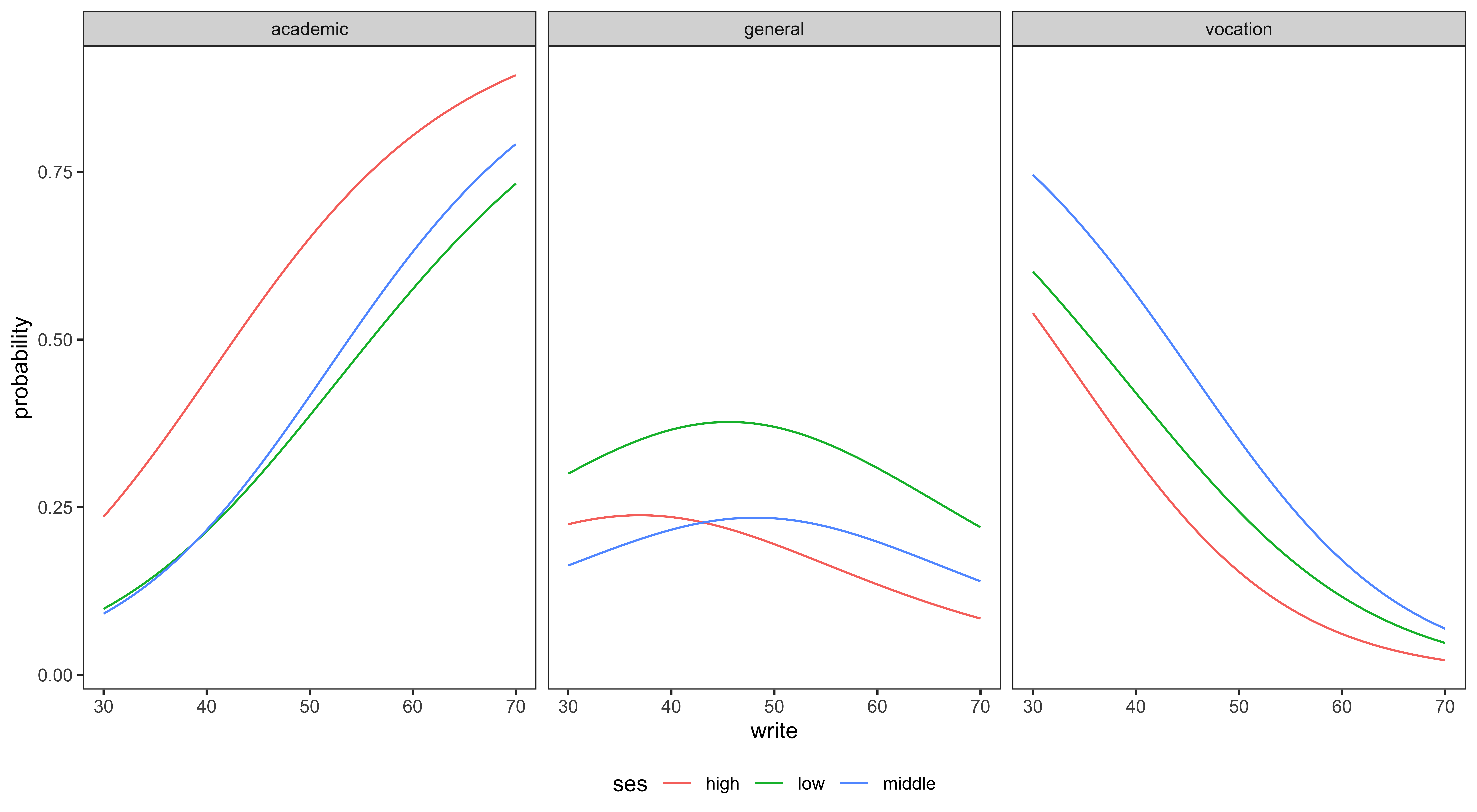
6     0.35    0.24     0.41

• Hold write at its mean and examine the predicted probabilities for each level of ses.

dses <- data.frame(ses = c("low", "middle", "high"), 
                   write = mean(multino_data$write))
predict(multino_fit, newdata = dses, type = "probs")

  academic general vocation
1     0.44    0.36     0.20
2     0.48    0.23     0.29
3     0.70    0.18     0.12

https://stackoverflow.com/questions/22905807/how-does-the-function-multinom-from-r-package-nnet-compute-the-multinomial-proba

Multinomial Logit - Probability Curve

Generalized Linear Models

Generalized Linear Models in Greater Generality

• Conditional on \(\mathbf{X}\), the response \(Y\) belongs to a certain family of distribution.¹
  • Linear regression: Gaussian
  • Logistic regression: Bernoulli, binomial, multinomial

• Model the mean of \(Y\) as a function of the predictors.
  • Linear regression: \(E(Y \mid \mathbf{x}) = \mathbf{x}'\boldsymbol \beta\)
  • Logistic regression: \(E(Y \mid \mathbf{x}) = P(Y=1 \mid \mathbf{x}) = \pi(\mathbf{x}) = \frac{e^{\mathbf{x}'\boldsymbol \beta}}{1 + e^{\mathbf{x}'\boldsymbol \beta}}\)

• In general, with \(E(Y \mid \mathbf{x}) = \mu\), the link function \(\eta(\mu) = {\bf x}'\boldsymbol \beta\) transforms \(\mu\) so that the transformed mean is a linear function of predictors!
  • Linear regression: \(\eta(\mu) = \mu\)
  • Logistic regression: \(\eta(\mu) = \log(\mu/(1-\mu))\)

Any regression approach that follows this general recipe is known as a generalized linear model (GLM).

1. Usually the distribution of \(Y\) belongs to the exponential family.

Link Function

• Logistic regression uses the logit function \(\eta = g(\pi) = \ln\left( \dfrac{\pi}{1-\pi}\right)\) as the link function.

• \(\pi = \dfrac{1}{1 + e^{-\eta}} \in (0, 1)\) is the CDF of the logistic distribution, whose PDF is of the from \[f(\eta) = \frac{e^{-\eta}}{(1 + e^{-\eta})^2}, \quad \eta \in(-\infty, \infty)\]

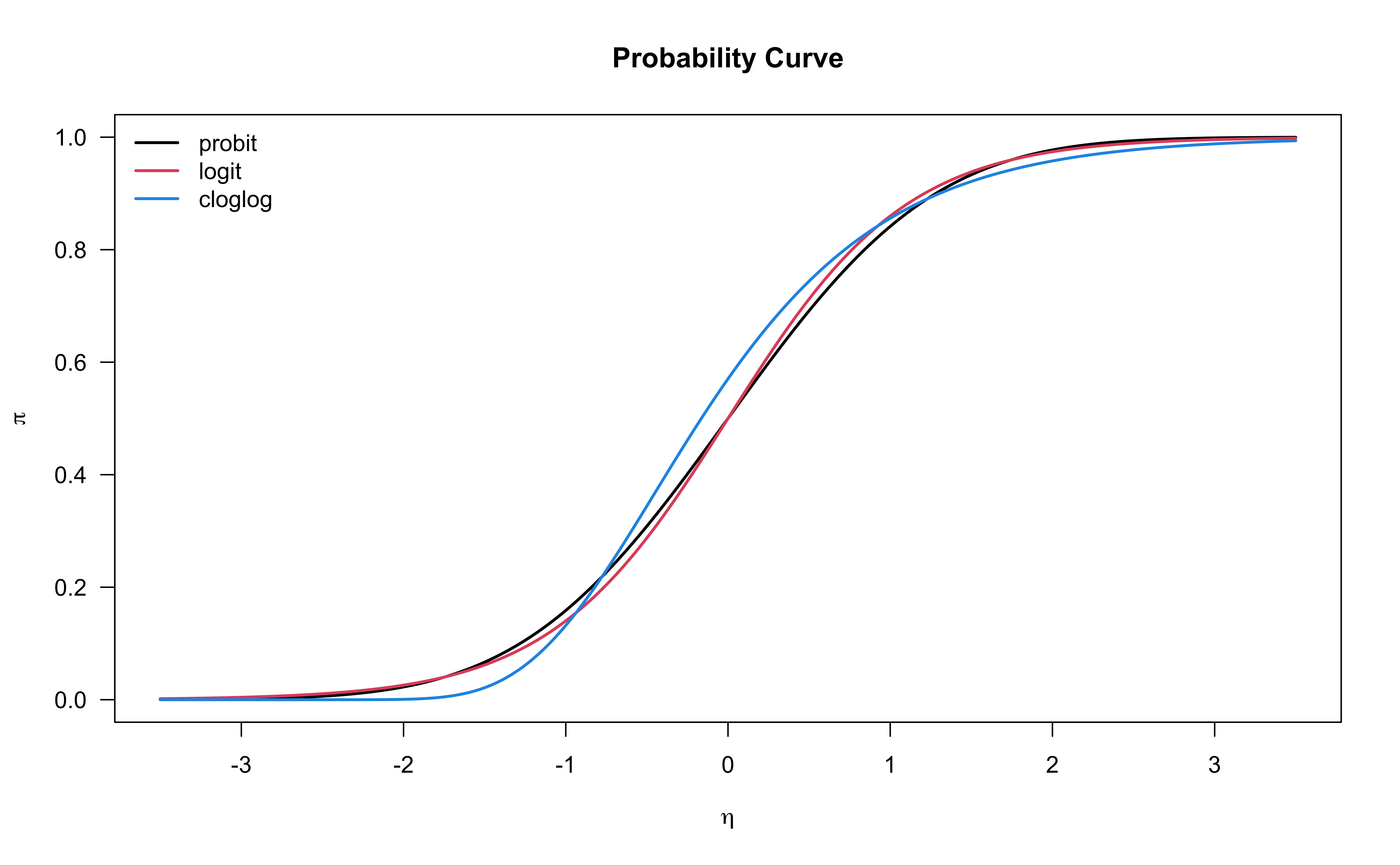
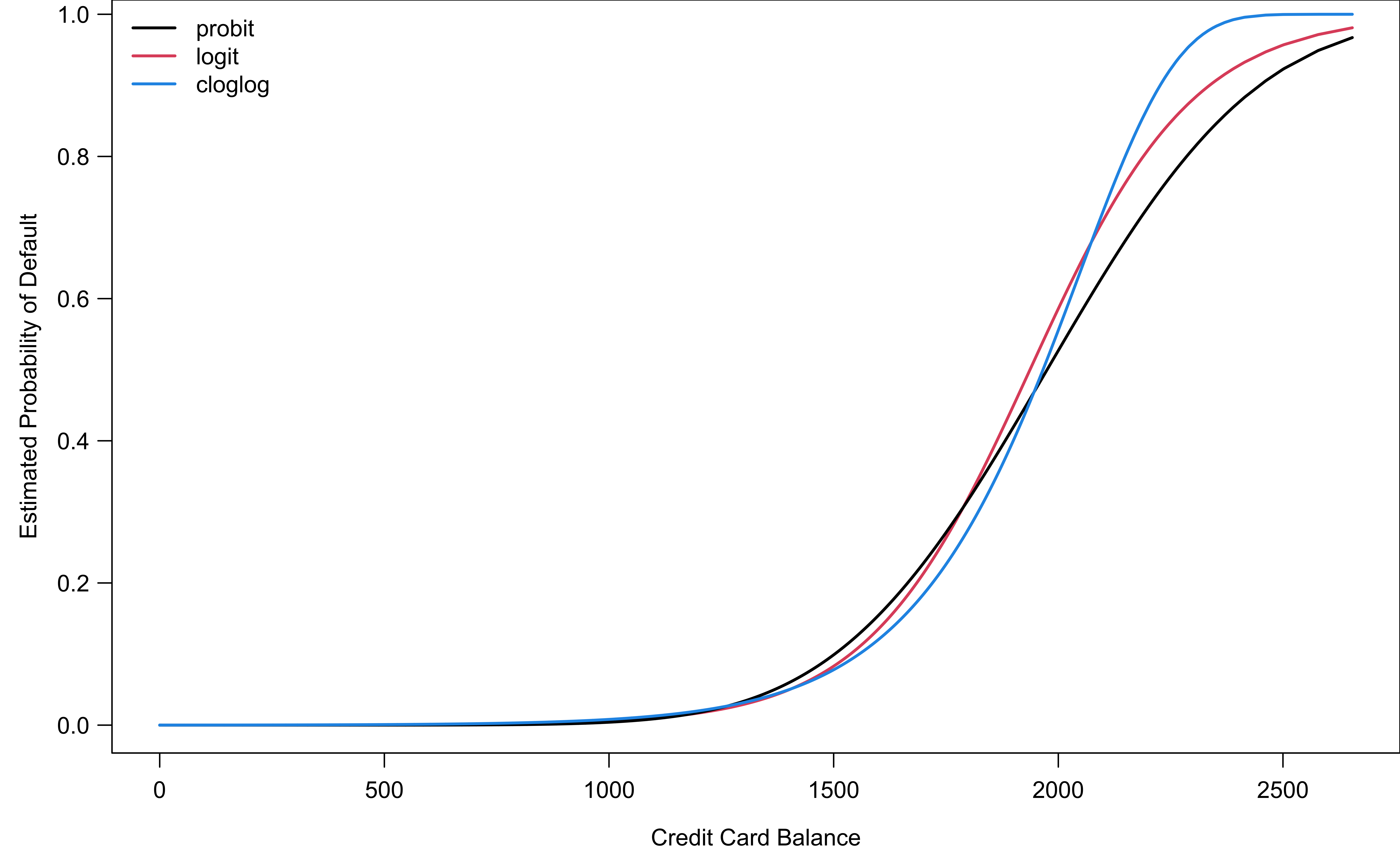
• Could use a different link function and hence CDF to describe the probability curve.

Probit and Complementary log-log (cloglog) Link

• If \(\pi = \Phi(\eta) \in (0, 1)\), \(\Phi(\cdot)\) is the CDF of standard normal distribution, the link function \[\eta = g(\pi) = \Phi^{-1}(\pi)\] is called probit, and the model is called probit model or probit regression.

• Another popular link function is the complementary log-log link: \[\eta = g(\pi) = \log\left( -\log(1-\pi)\right)\] where \(\pi = 1 - \exp(-\exp(\eta))\) is the CDF of the so called Gumbel distribution.¹

1. The complementary log-log link is actually defined by a negative Gumbel random variable. No worries about why it is used at this moment.

Link Function Summary

Distribution	Link Function \(\eta = g(\pi)\)	CDF \(\pi = g^{-1}(\eta)\)	PDF
Logistic	logit: \(\ln\left( \dfrac{\pi}{1-\pi}\right)\)	\(\dfrac{1}{1 + e^{-\eta}}\)	\(\dfrac{e^{-\eta}}{(1 + e^{-\eta})^2}\)
Normal	probit: \(\Phi^{-1}(\pi)\)	\(\Phi(\eta)\)	\(\frac{1}{\sqrt{2\pi}} e^{-\frac{\eta^2}{2}}\)
Gumbel	cloglog: \(\log\left( -\log(1-\pi)\right)\)	\(1 - \exp(-\exp(\eta))\)	\(e^{-(\eta + e ^ {-\eta})}\)

Any transformation that maps probabilities into the real line could be used to produce a GLM for binary classification, as long as the transformation is one-to-one continuous and differentiable.

\[\pi = F(\eta)\] \[\eta = F^{-1}(\pi)\]

Link Function Summary

Name	Link Function \(\eta = g(\pi)\)
logit	\(\ln\left( \dfrac{\pi}{1-\pi}\right)\)
probit	\(\Phi^{-1}(\pi)\)
cloglog	\(\log\left( -\log(1-\pi)\right)\)

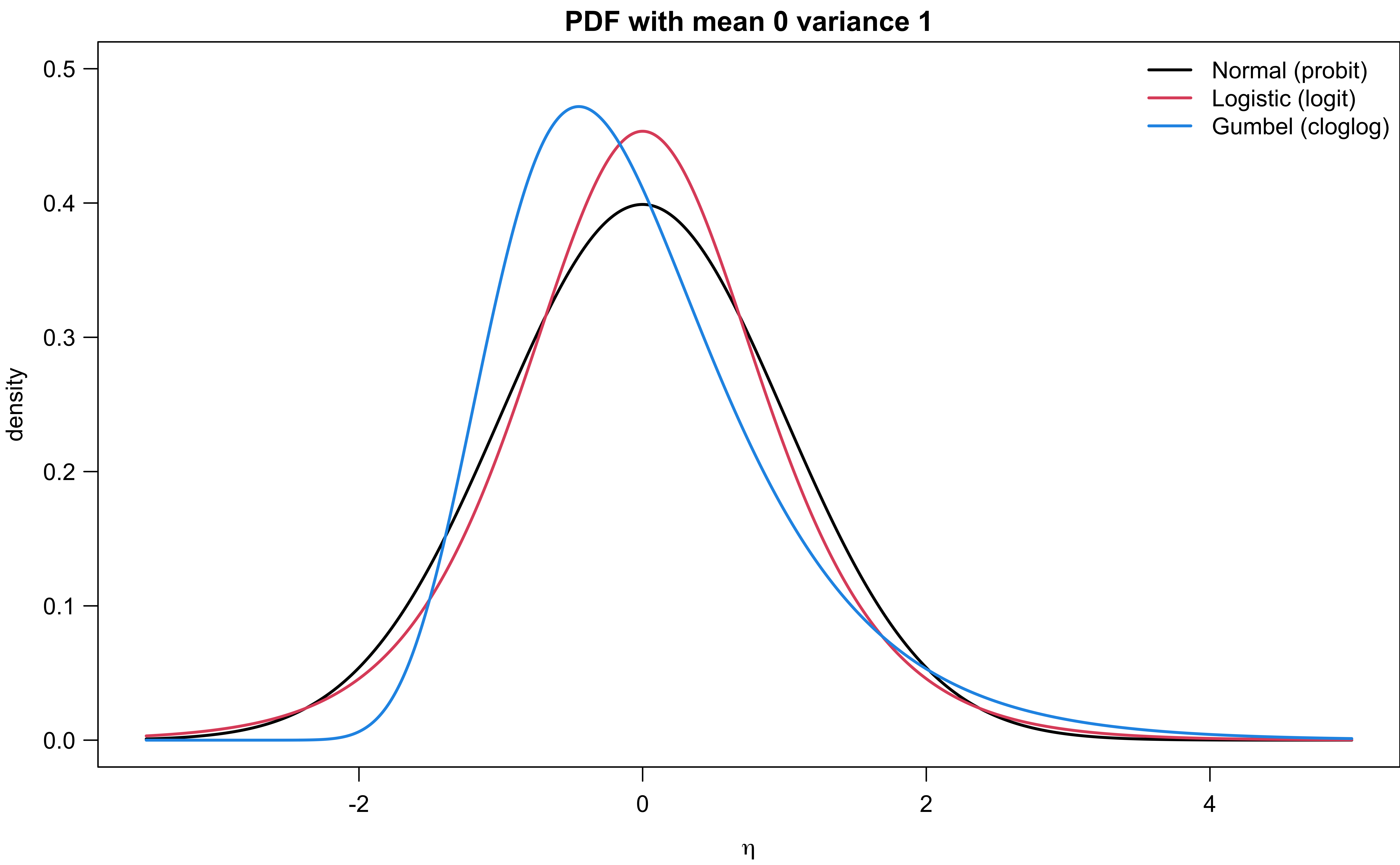
• Logit and probit links produce similar curve. For simple regression, both estimate \(\pi = 1/2\) when \(x = -\beta_0/\beta_1\) and exhibit symmetric behavior.
• The complementary log-log link is not symmetric.

PDF

• Normal and logistic density are symmetric, while Gumbel is right skewed.

Probability Curve

Probit and Complementary log-log Links

probit_fit <- glm(default ~ balance, data = Default, family = binomial(link = "probit"))
cloglog_fit <- glm(default ~ balance, data = Default, family = binomial(link = "cloglog"))

Other Topics

• Repeated measures and binomial logistic regression

• Regression diagnostics for binary data

• Penalized logistic regression

• Exponential family

• Poisson regression

https://grodri.github.io/glms/

https://stats.oarc.ucla.edu/r/dae/multinomial-logistic-regression/

https://glmnet.stanford.edu/articles/glmnet.html