Tree-based Methods
MSSC 6250 Statistical Machine Learning
Department of Mathematical and Statistical Sciences
Marquette University
Tree-based Methods
Can be used for regression and classification.
IDEA: Segmenting the predictor space into many simple regions.
Simple, useful for interpretation, and has nice graphical representation.
Not competitive with the best supervised learning approaches in terms of prediction accuracy. (Large bias)
Combining a large number of trees (ensembles) often results in improvements in prediction accuracy, at the expense of some loss interpretation.
Decision Trees: Classification and Regression Trees (CART)
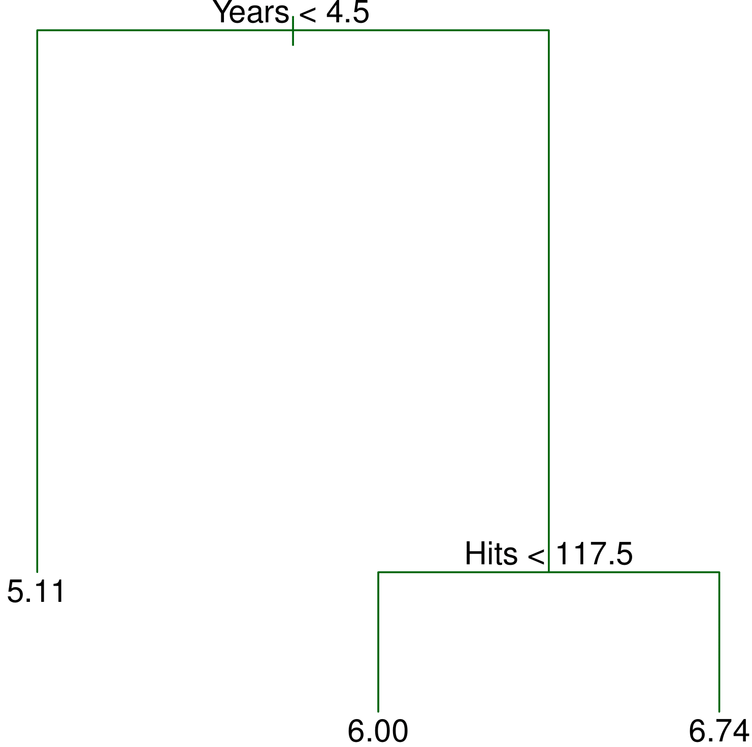
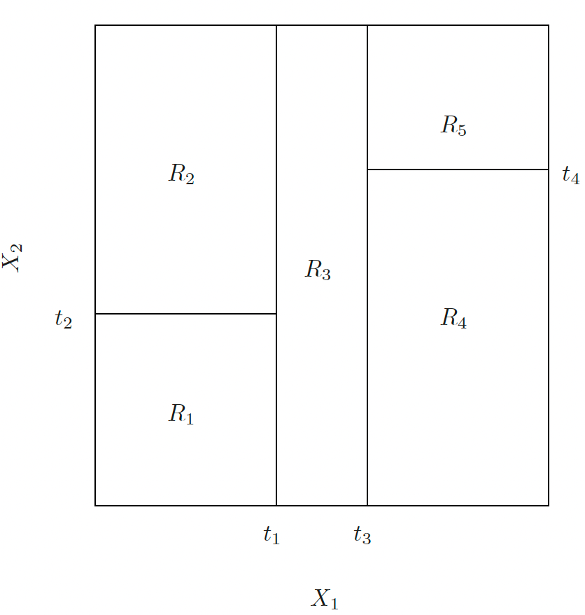
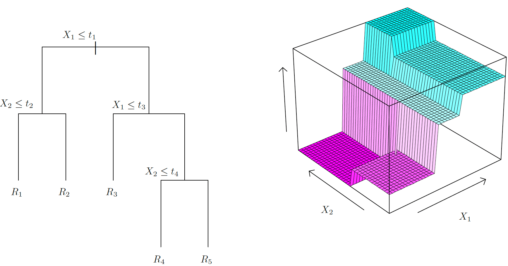
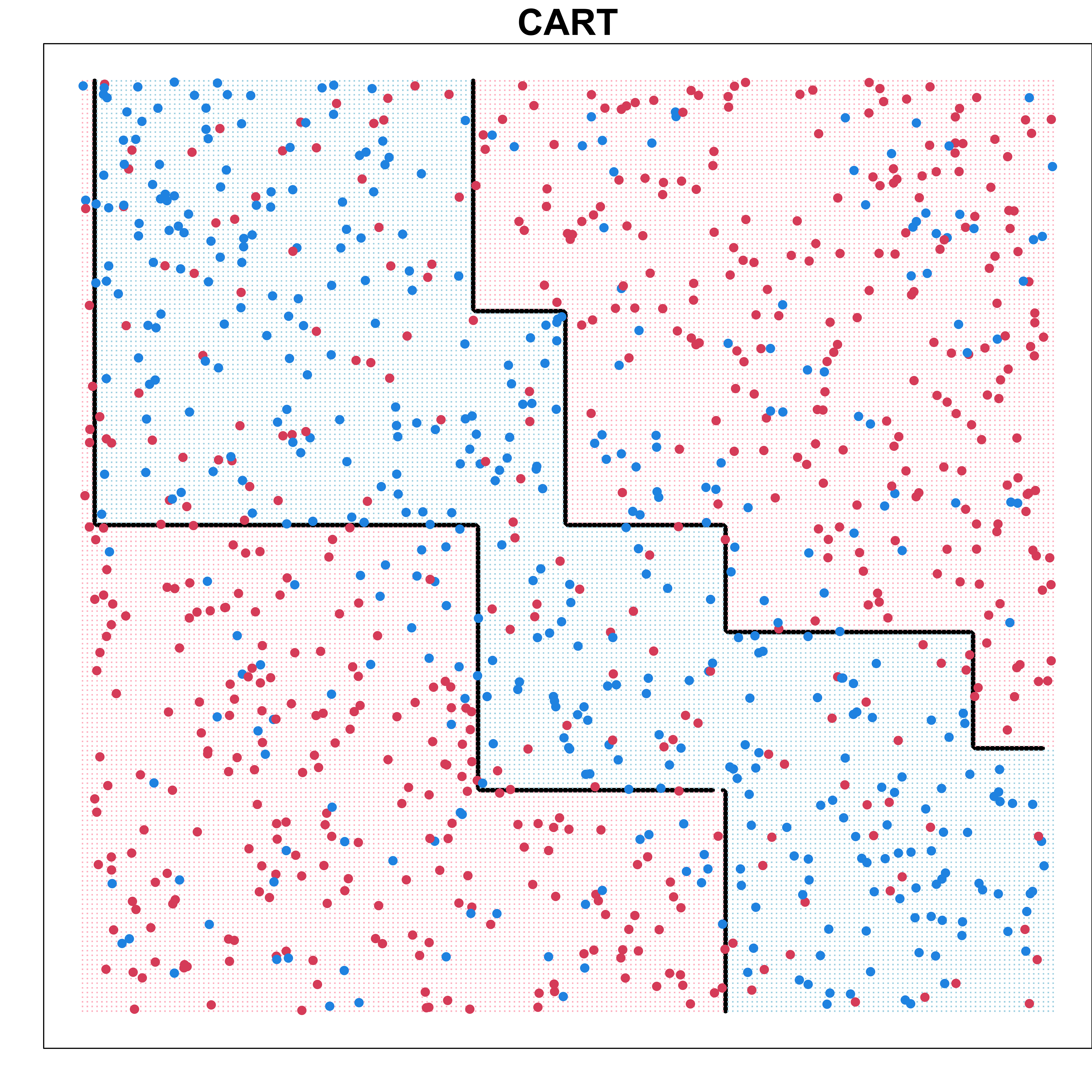
CART is a nonparametric method that recursively partitions the feature space into hyper-rectangular subsets (boxes), and make prediction on each subset.
Divide the predictor space — the set of possible values for \(X_1, X_2, \dots, X_p\) — into \(J\) distinct and non-overlapping regions, \(R_1, R_2, \dots, R_J\).
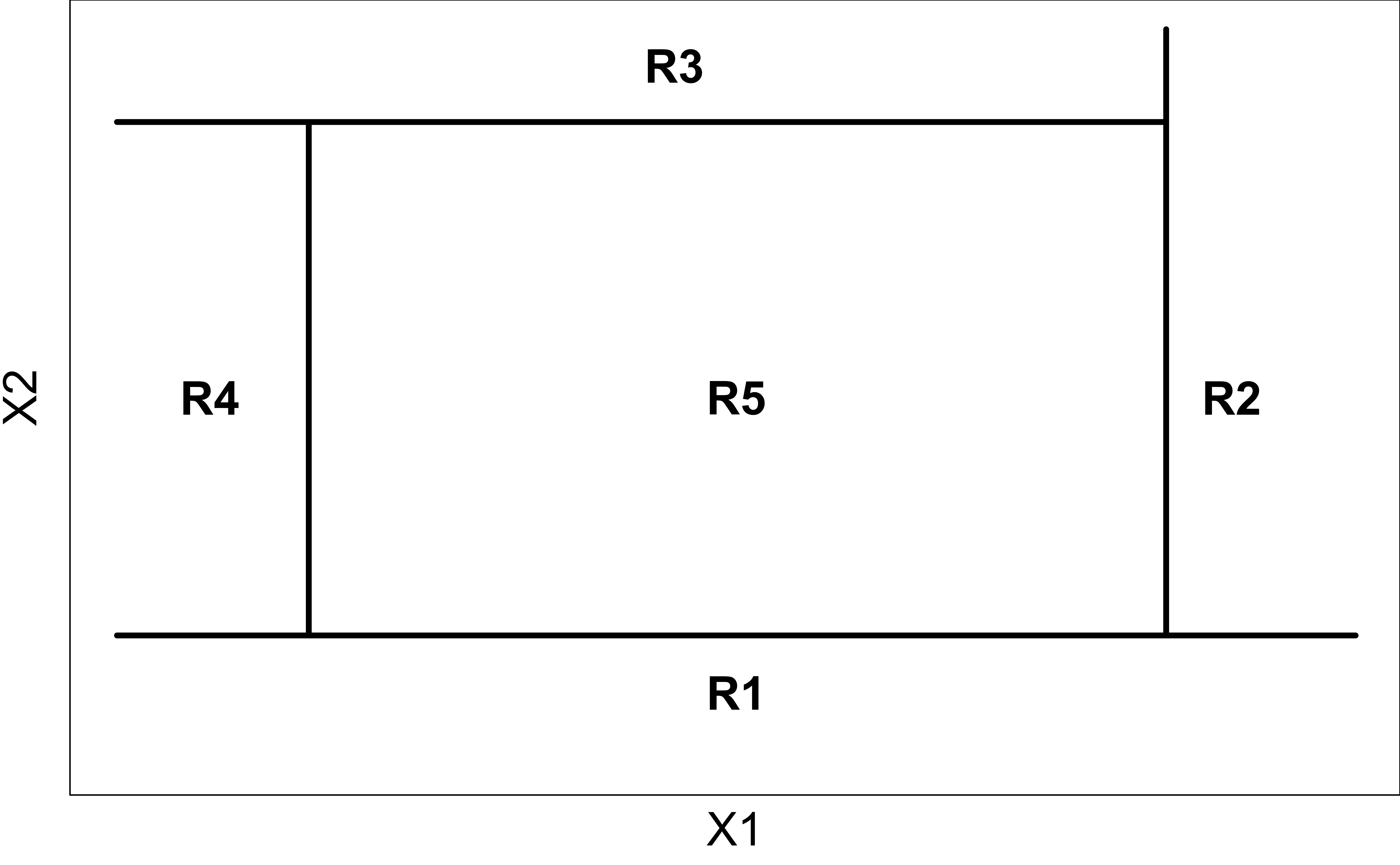
- For every test point that falls into the region \(R_j\) , we make the same prediction:
- Regression: the mean of the response values for the training points in \(R_j\), i.e., \(\hat{y}_{R_j} = \sum_{k \in R_j} y_k / |R_j|\)
- Classification: the most commonly occurring class of training points in \(R_j\), i.e., \(\hat{y}_{R_j} = \underset{c}{\text{arg max}} \, \,\# (y_k = c)\), \(y_k \in R_j\).
Recursive Binary Splitting
- Computationally infeasible to consider every possible partition of the feature space into arbitrary \(J\) boxes.
- The recursive binary splitting is top-down and greedy:
- Top-down: begins at the top of the tree (the entire \(X\) space)
- Greedy: at each step, the best split is made at that particular step, rather than looking ahead and picking a split that will lead to a better tree in some future step.
- Select \(X_j\) and a cutoff \(s\) so that splitting the predictor space into \(\{\mathbf{X}\mid X_j < s \}\) and \(\{\mathbf{X}\mid X_j \ge s \}\) leads to the greatest reduction in
- \(SS_{res}\) for regression
- Gini index, entropy or misclassification rate for classification
- Repeatedly split one of the two previously identified regions until a stopping criterion is reached.
Classification Tree
KNN requires K and a distance measure.
SVM requires kernels.
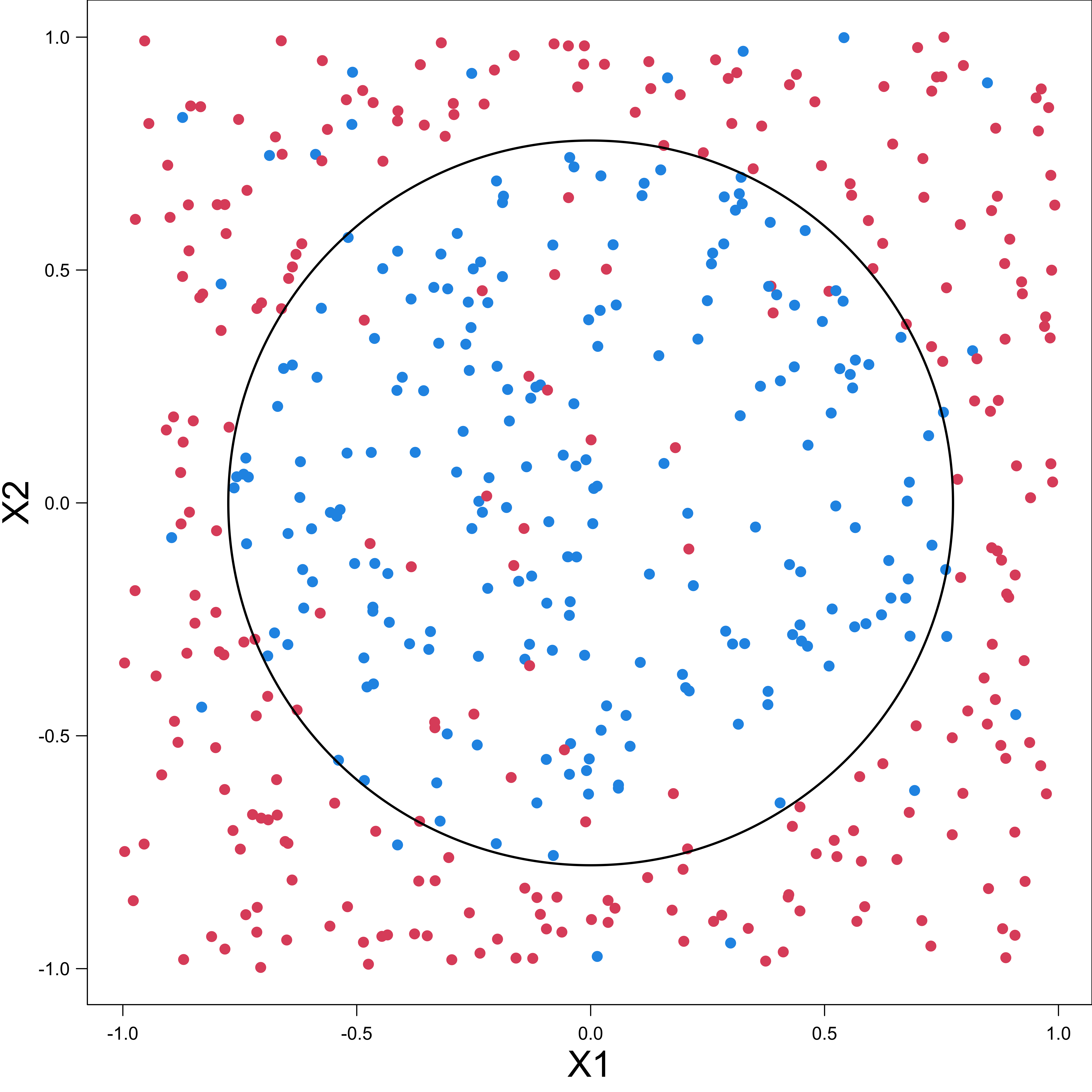
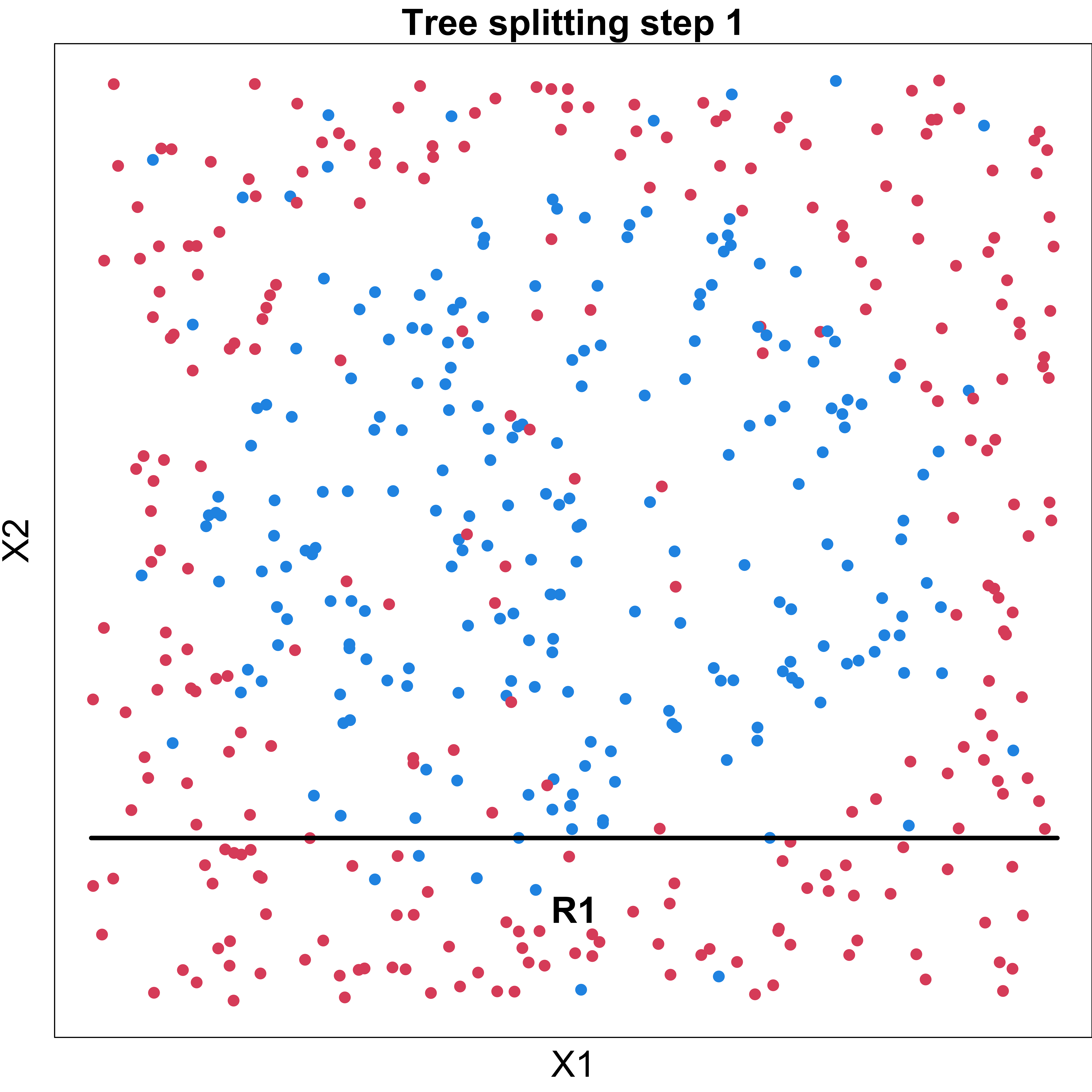
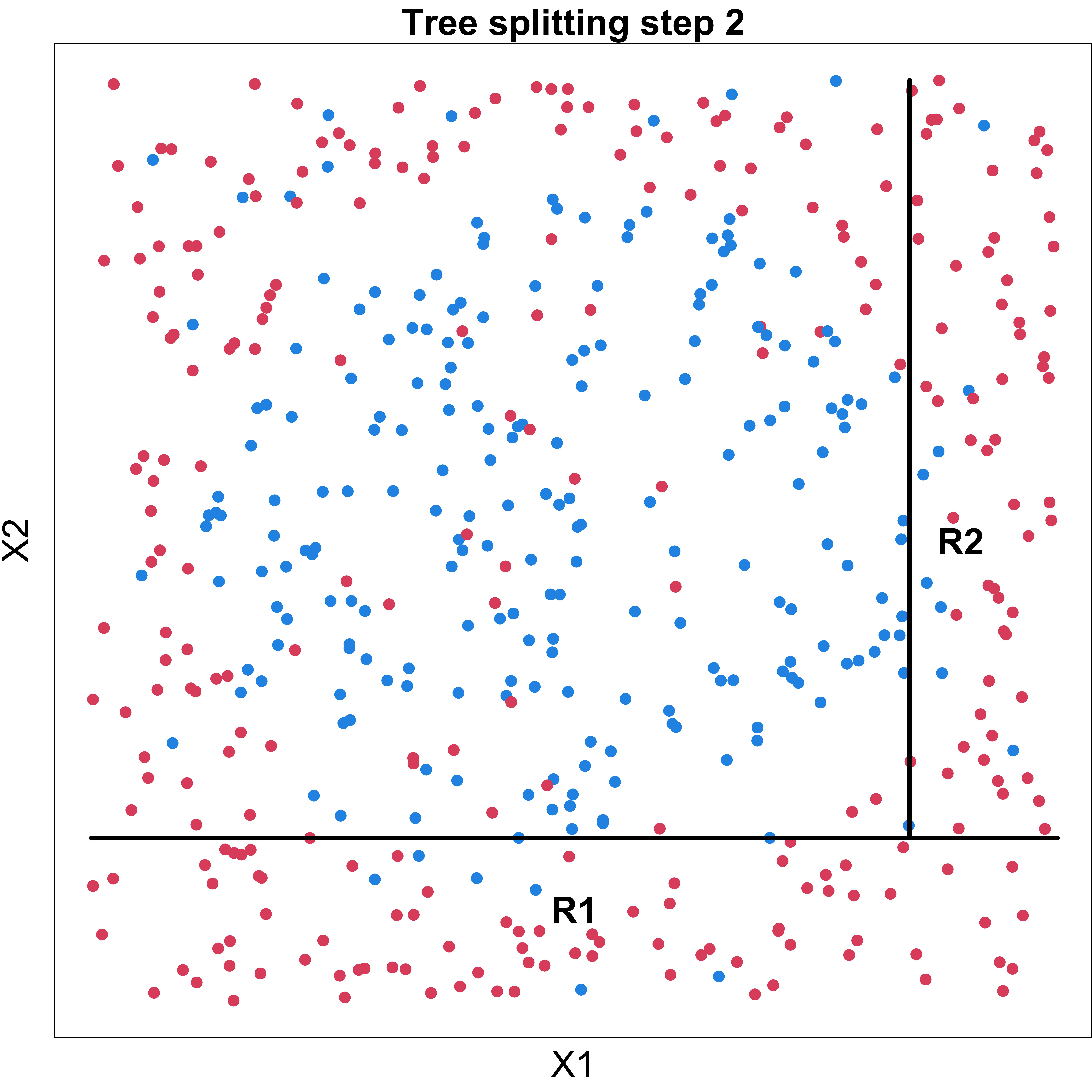
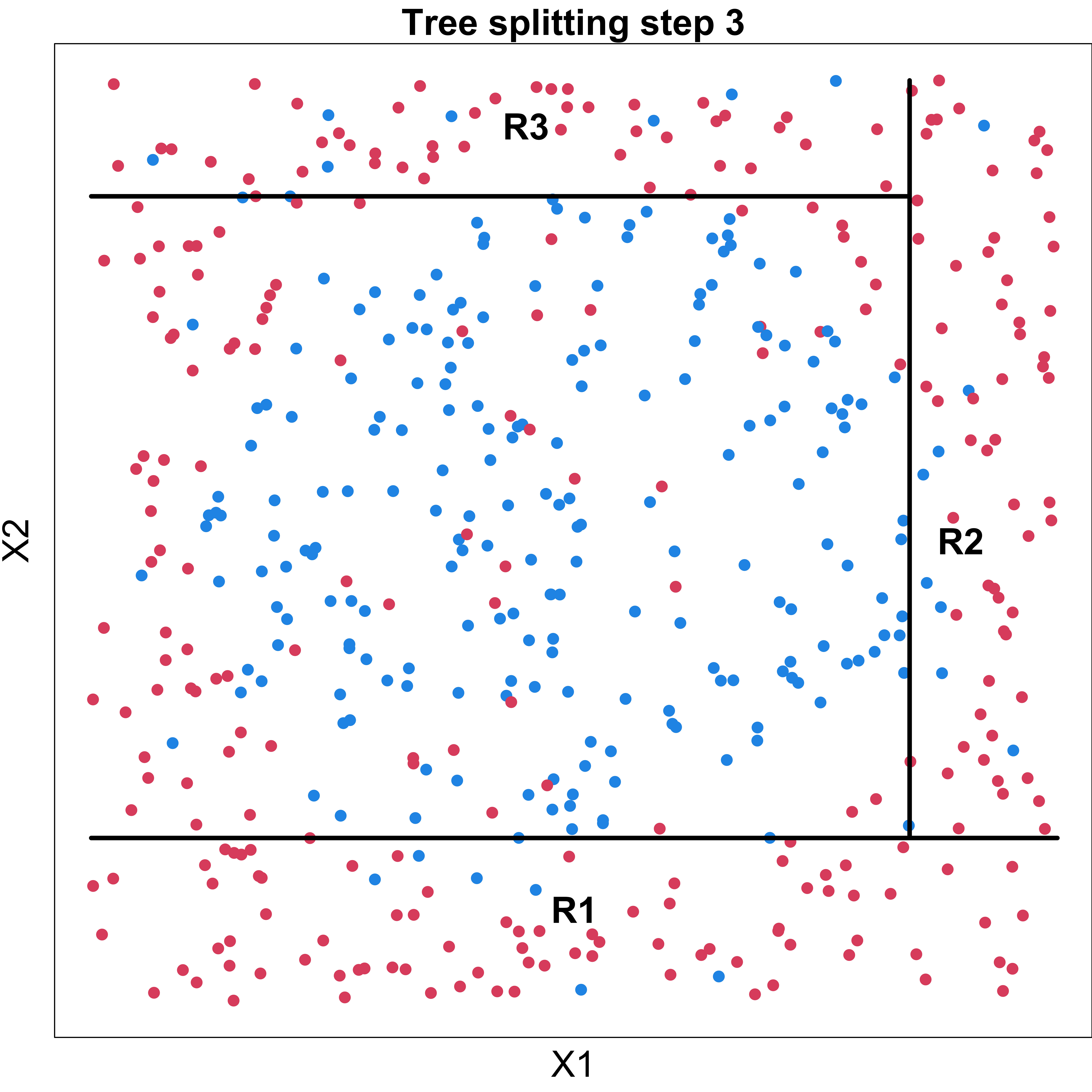
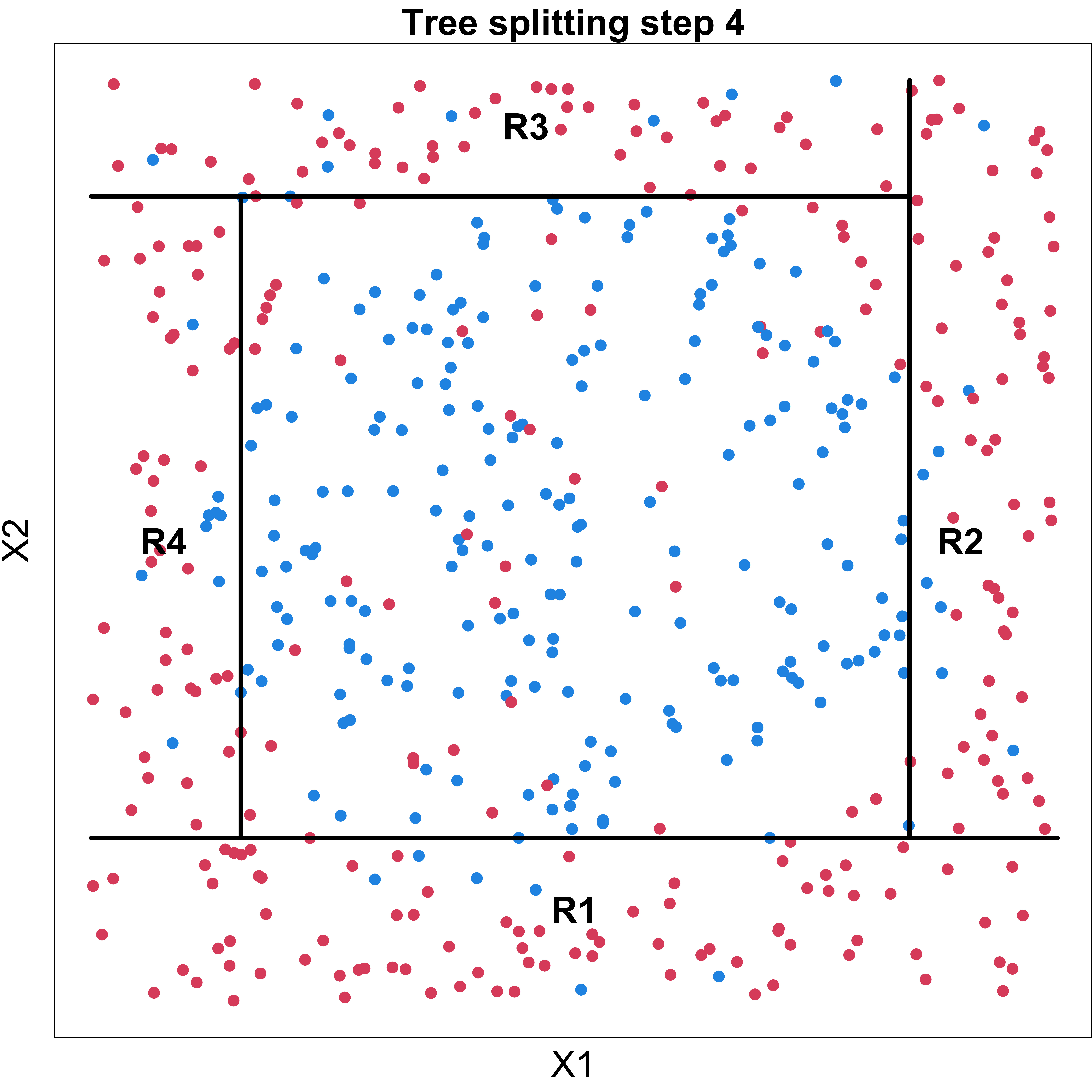
Tree solves this by recursively partitioning the feature space using a binary splitting rule \(\mathbf{1}\{x \le c \}\)
0: Red; 1: Blue
Classification Tree
If \(x_2 < -0.64\), \(y = 0\).
Classification Tree
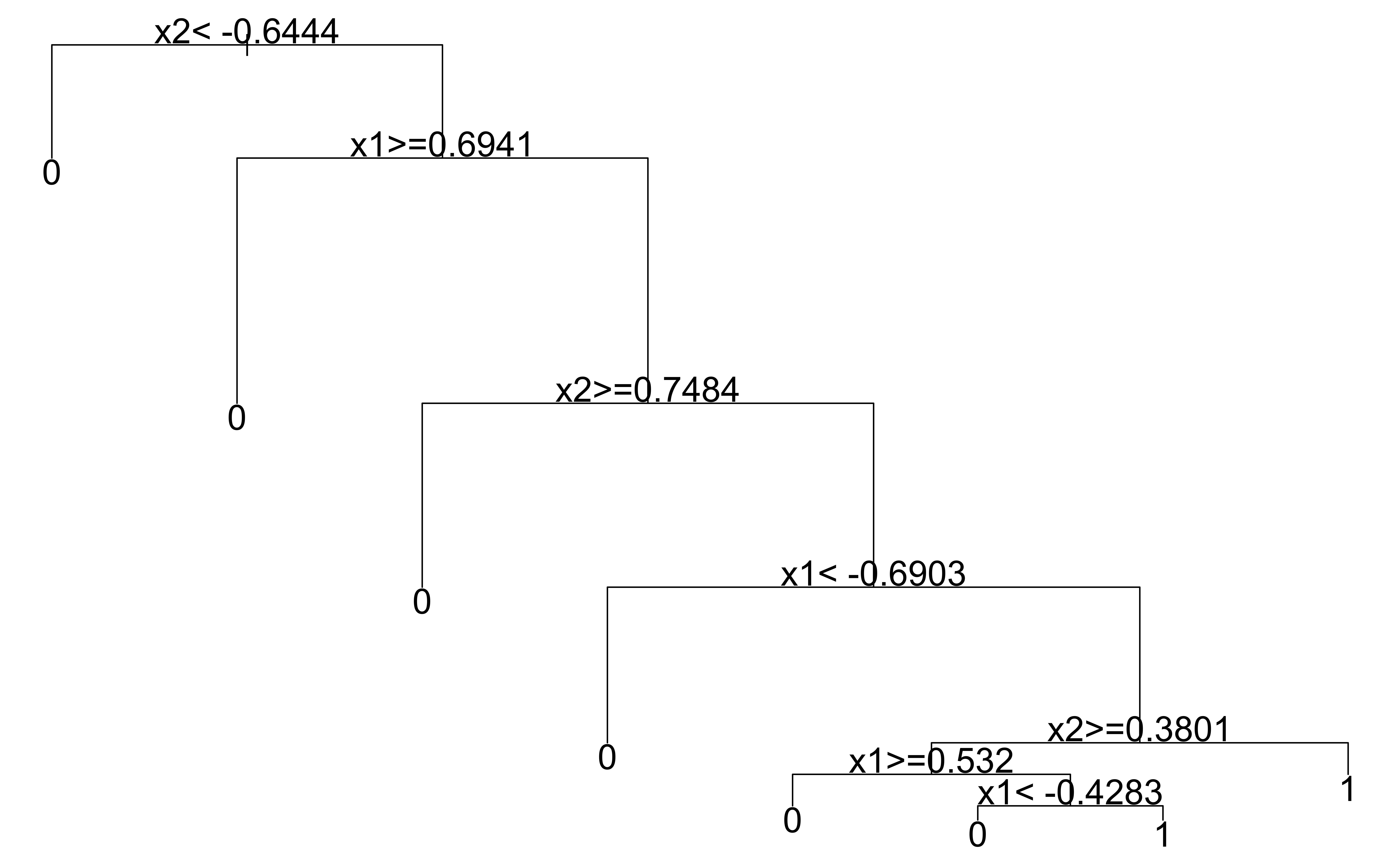
If \(x_2 \ge -0.64\) and \(x_1 \ge 0.69\), \(y = 0\).

Classification Tree
If \(x_2 \ge -0.64\), \(x_1 < 0.69\), and \(x_2 \ge 0.75\), \(y = 0\).

Classification Tree
If \(x_2 \ge -0.64\), \(x_1 < 0.69\), \(x_2 < 0.75\), and \(x_1 < -0.69\), \(y = 0\).

Classification Tree
Step 5 may not be beneficial.

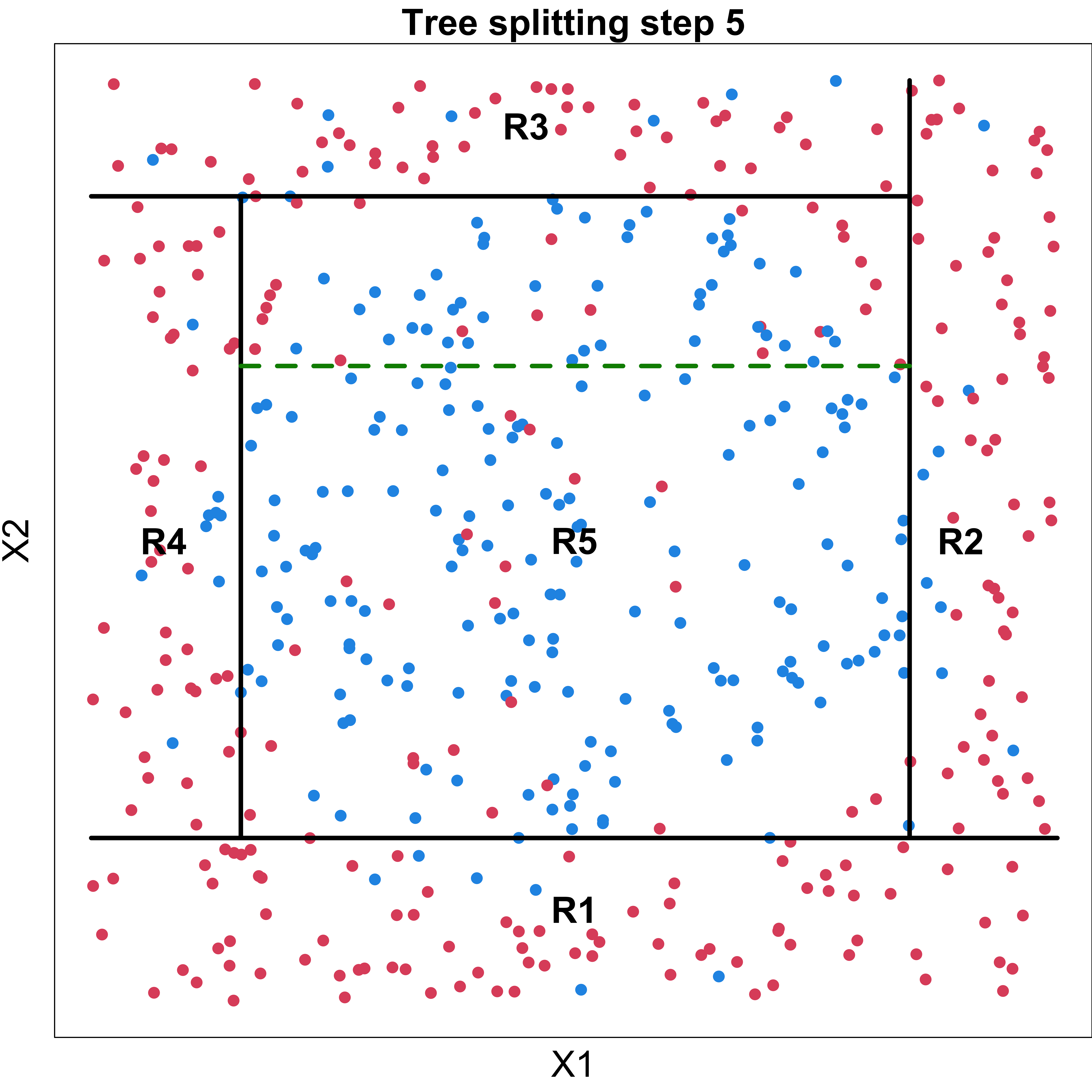
Classification Tree
Step 6 may not be beneficial. (Could overfit)

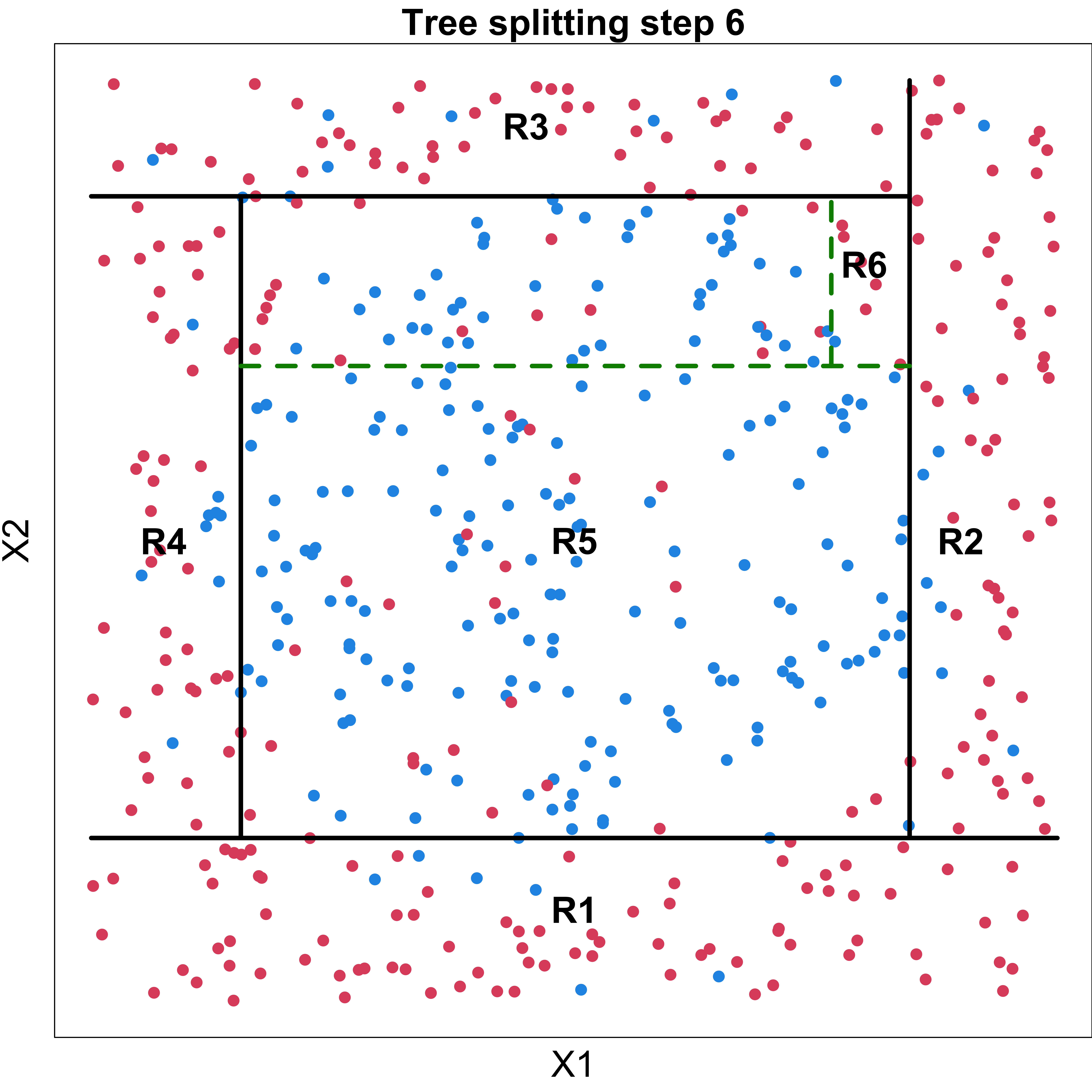
Classification Tree
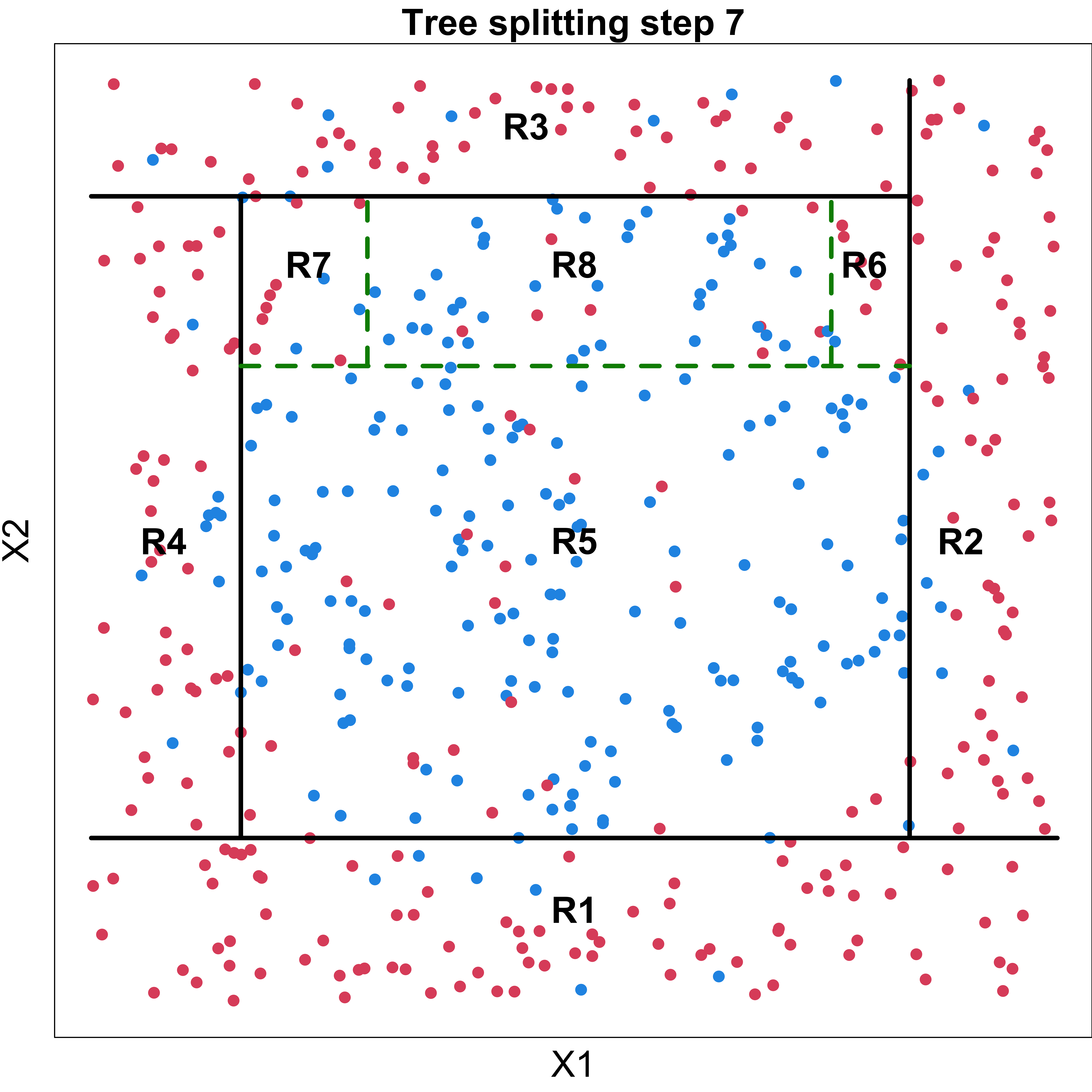
Step 7 may not be beneficial. (Could overfit)

Misclassification Rate
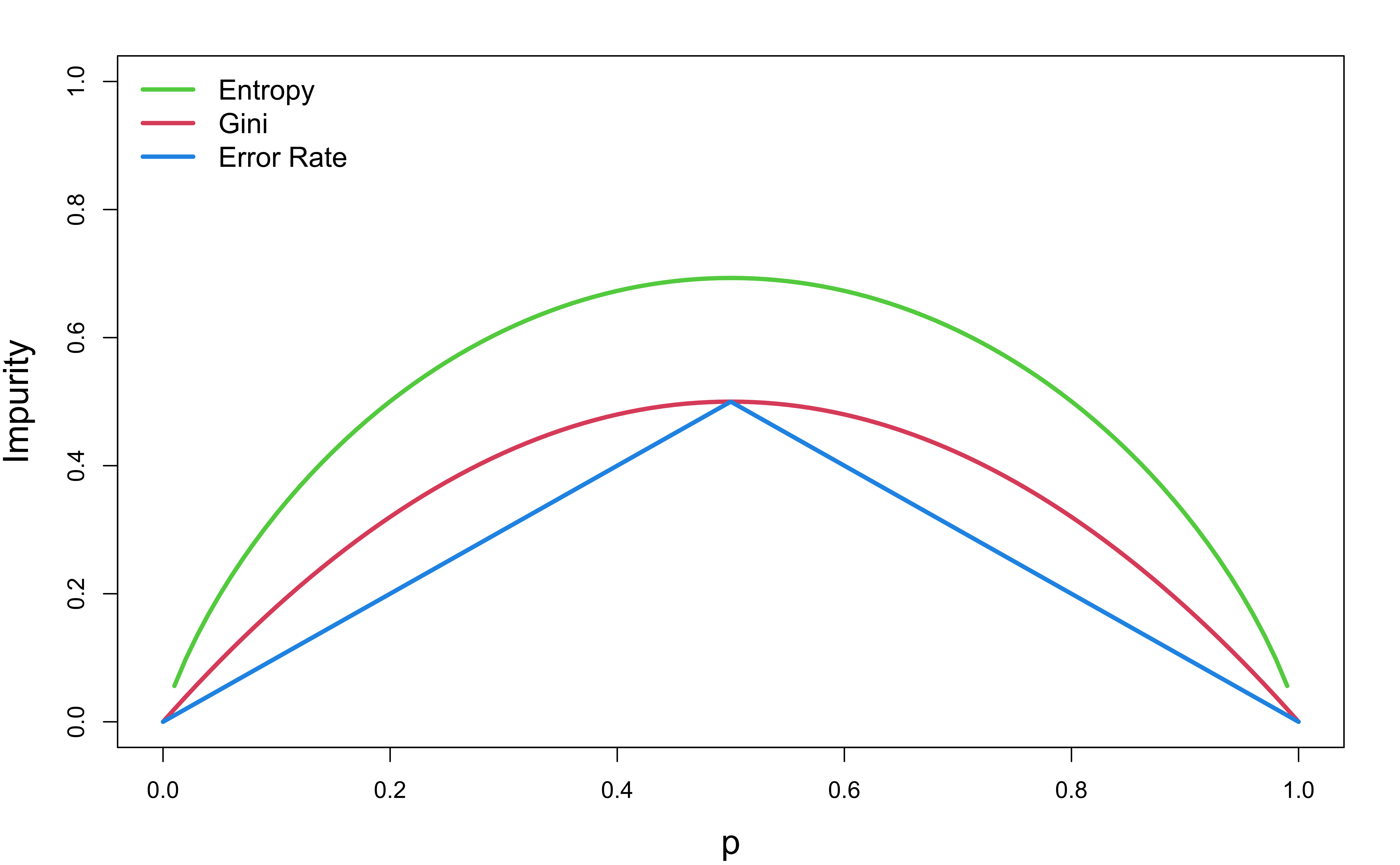
The classification error rate is the fraction of the training observations in the region that do not belong to the most common class: \[1 - \max_{k} (\hat{p}_{mk})\] where \(\hat{p}_{mk}\) is the proportion of training observations in the \(m\)th region that are from the \(k\)th class.
It is not sensitive for tree-growing.
Hope to have nodes (regions) including training points that belong to only one class.
Gini Index (Impurity)
The Gini index is defined by
\[\sum_{k=1}^K \hat{p}_{mk}(1 - \hat{p}_{mk})\] which is a measure of total variance across the \(K\) classes.
Gini is small if all of the \(\hat{p}_{mk}\)s are close to zero or one.
Node purity: a small value indicates that a node contains predominantly observations from a single class.
Shannon Entropy
The Shannon entropy is defined as
\[- \sum_{k=1}^K \hat{p}_{mk} \log(\hat{p}_{mk}).\]
The entropy is near zero if the \(\hat{p}_{mk}\)s are all near zero or one.
Gini index and the entropy are similar numerically.
Comparing Measures
- Use Gini and Entropy for training (building a tree), and use error rate for evaluating predictive accuracy.
Regression Tree
The goal is to find boxes \(R_1, \dots ,R_J\) that minimize the \(SS_{res}\), given by \[\sum_{j=1}^J\sum_{i \in R_j}\left( y_i - \hat{y}_{R_j}\right)^2\] where \(\hat{y}_{R_j}\) is the mean response for the training observations within \(R_j\).
Tree Pruning
- Using regression and classification performance measures to grow trees with no penalty on the tree size leads to overfitting.
- Cost complexity pruning:
Given the largest tree \(T_{max}\),
\[\begin{align} \min_{T \subset T_{max}} \sum_{m=1}^{|T|}\sum_{i:x_i\in R_m} \left( y_i - \hat{y}_{R_m}\right)^2 + \alpha|T| \end{align}\] where \(|T|\) indicates the number of terminal nodes of the tree \(T\).
Large \(\alpha\) results in small trees
Choose \(\alpha\) using CV
Algorithm 8.1 in ISL for building a regression tree.
For classification, replace \(SS_{res}\) with a classification performance measure.
Implementation
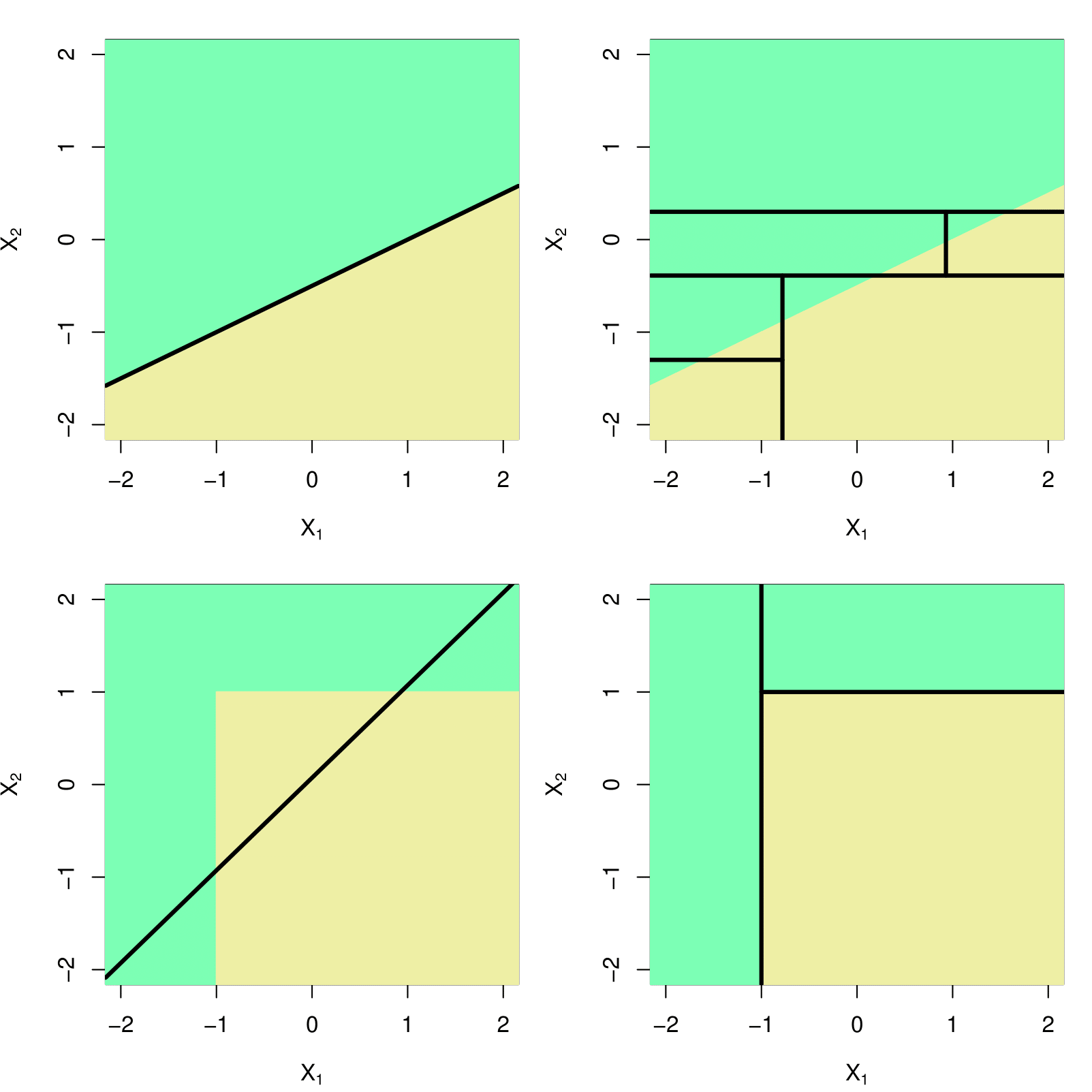
Trees v.s. Linear Regression
Linear regression
\[f(X) = \beta_0 + \sum_{j=1}^pX_j\beta_j\]
- Performs better when the relationship between \(y\) and \(x\) is approximately linear.
Regression tree
\[f(X) = \sum_{j=1}^J \hat{y}_{R_j}\mathbf{1}(\mathbf{X}\in R_j)\]
Performs better when there is a highly nonlinear and complex relationship between \(y\) and \(x\).
Preferred for interpretability and visualization.
Trees v.s. Linear Models
Ensemble Learning: Bagging, Random Forests, Boosting
Two heads are better than one, not because either is infallible, but because they are unlikely to go wrong in the same direction. – C.S. Lewis, British Writer (1898 - 1963)
『三個臭皮匠,勝過一個諸葛亮』
Ensemble Methods
An ensemble method combines many weak learners (unstable, less accurate) to obtain a single and powerful model.
The CARTs suffer from high variance.
If independent \(Z_1, \dots, Z_n\) have variance \(\sigma^2\), then \(\bar{Z}\) has variance \(\sigma^2/n\).
Averaging a set of observations reduces variance!
With \(B\) separate training sets,
\[\hat{f}_{avg}(x) = \frac{1}{B}\sum_{b=1}^B\hat{f}_{b}(x)\]
Bagging
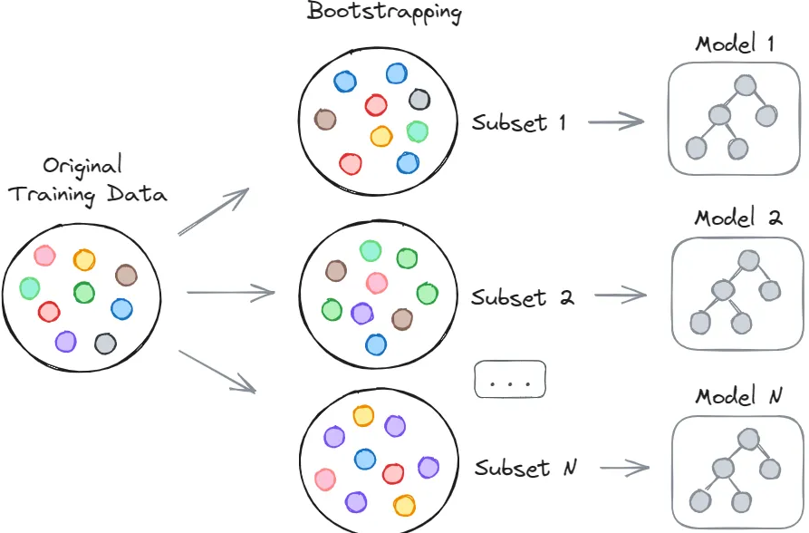
- Bootstrap aggregation, or bagging is a procedure for reducing variance.
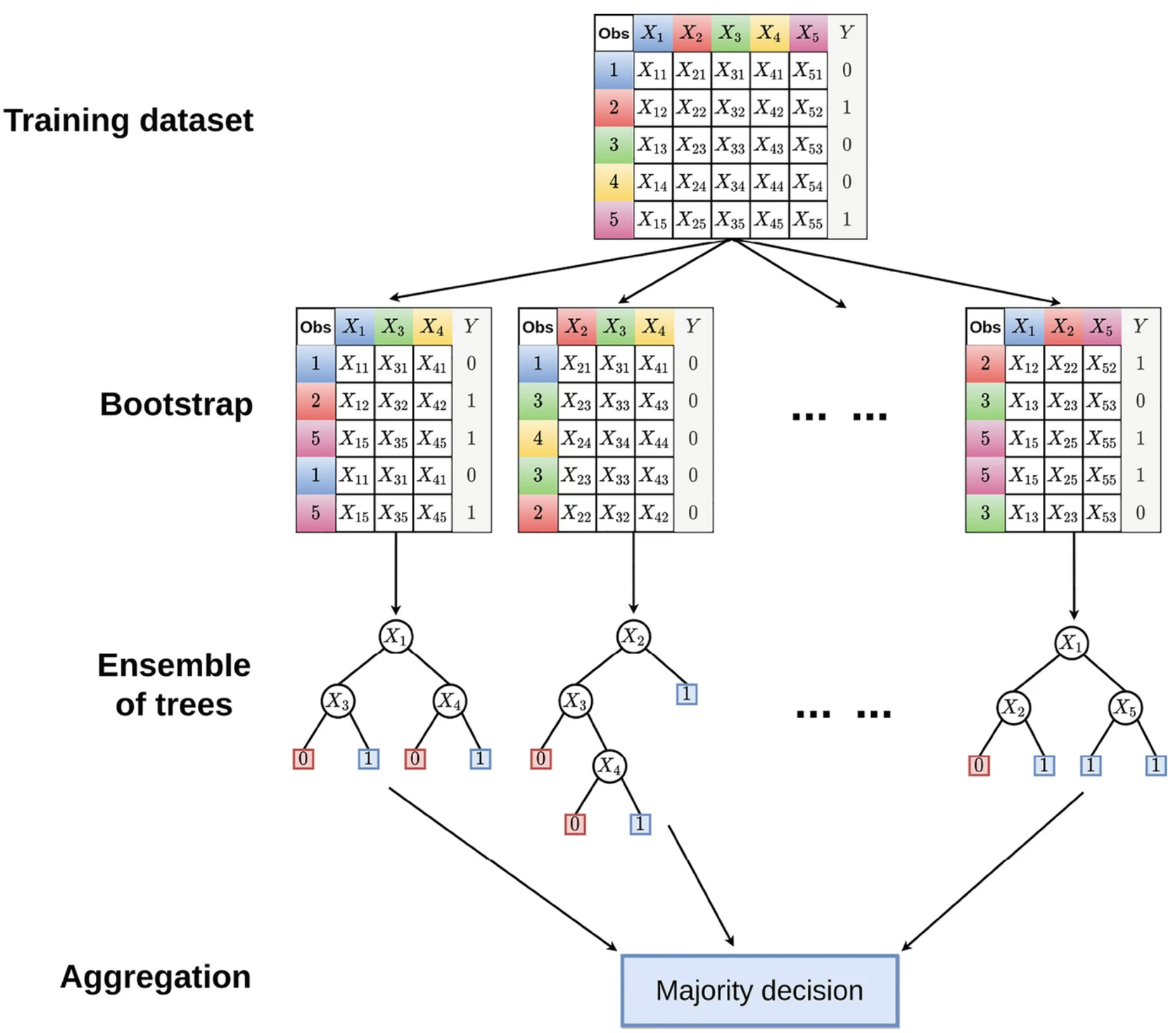
- Generate \(B\) bootstrap samples by repeatedly sampling with replacement from the training set \(B\) times.
\[\hat{f}_{bag}(x) = \frac{1}{B}\sum_{b=1}^B\hat{f}^*_{b}(x)\]
Bagging on Decision Trees

CART v.s. Bagging
For CART, the decision line has to be aligned to axis.
For Bagging, \(B = 200\) each having 400 training points. Boundaries are smoother.
Notes of Bagging
Using a large \(B\) will not lead to overfitting.
Use \(B\) sufficiently large that the error has settled down.
Bagging improves prediction accuracy at the expense of interpretability.
-
When different trees are highly correlated, simply averaging is not very effective.
- If there is one very strong predictor, in the collection of bagged trees, all of the trees will use this strong predictor in the top split. Therefore, all of the bagged trees will look similar to each other.
The predictions from the bagged trees will be highly correlated, and hence averaging does not lead to as large reduction in variance.
Random Forests
Random forests improve bagged trees by decorrelating the trees.
\(m\) predictors are randomly sampled as split candidates from the \(p\) predictors.
Random Forests
\(m \approx \sqrt{p}\) for classification; \(m \approx p/3\) for regression.
Decorrelating: on average \((p − m)/p\) of the splits will not even consider the strong predictor, and so other predictors will have more of a chance.
If \(m = p\), random forests = bagging.
The improvement is significant when \(p\) is large.
CART vs. Bagging vs. Random Forests
-
randomForest::randomForest(x, y, mtry, ntree, nodesize, sampsize)
Boosting
Bagging
Trees are built on independent bootstrap data sets.
Trees are grown deep.
Large number of trees (\(B\)) won’t overfit.
Boosting
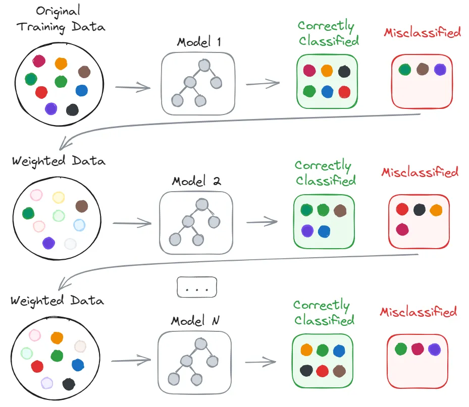
Trees are grown sequentially: each tree is grown using information from previously grown trees.
Each tree is fit on a modified version of the original data set, the residuals/false predictions!
Trees are rather small (weak learner).
Large \(B\) can overfit.
Boosting
Boosting for Classification
-
distribution = "bernoulli": LogitBoost
gbm.fit = gbm::gbm(y ~ ., data = data.frame(x1, x2, y),
                   distribution = "bernoulli",
                   n.trees = 10000, shrinkage = 0.01, bag.fraction = 0.6,
                   interaction.depth = 2, cv.folds = 10)
Boosting Cross Validation
gbm.perf(gbm.fit, method = "cv")[1] 1181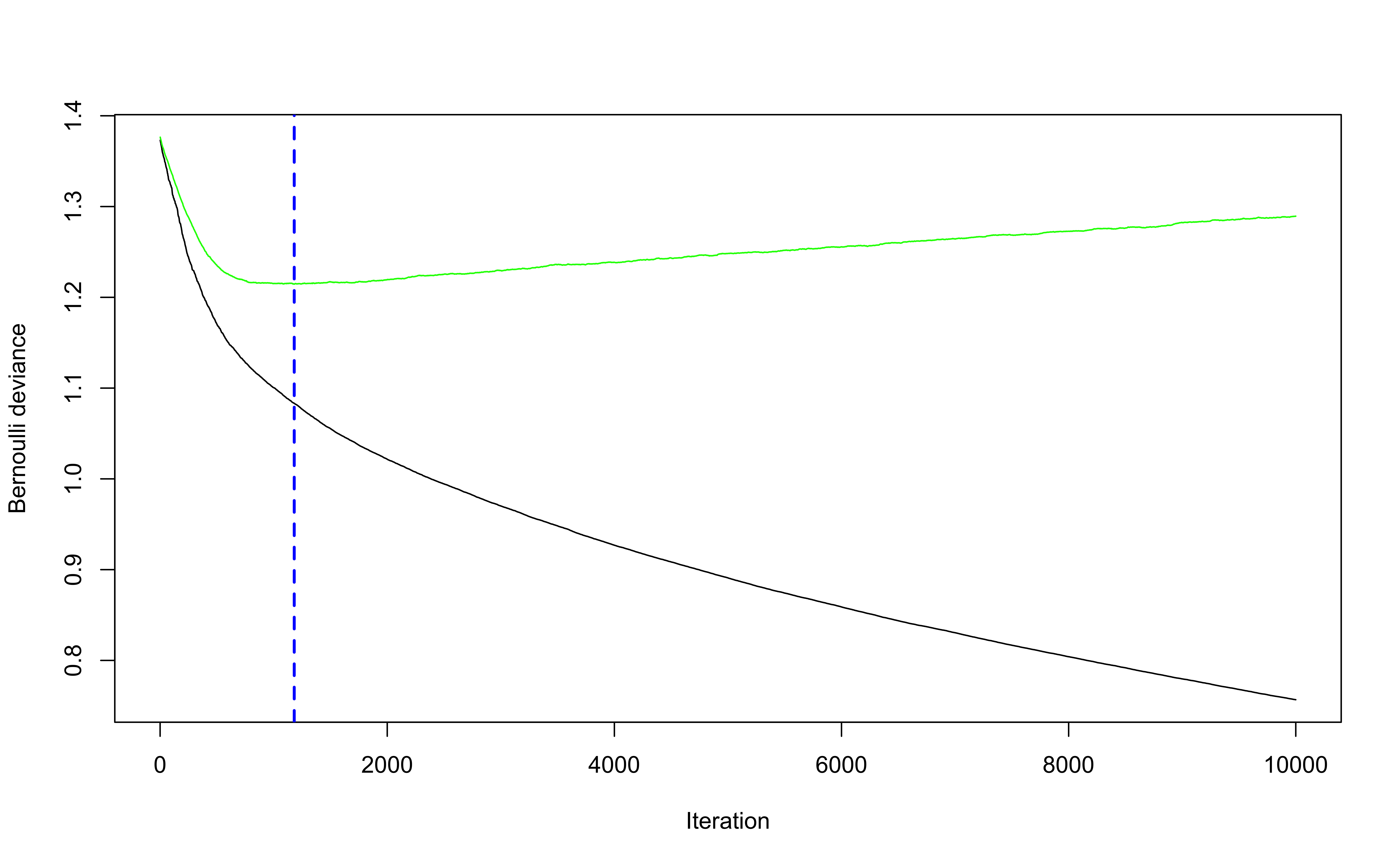
Boosting for Regression
gbm.fit <- gbm::gbm(y ~ x, data = data.frame(x, y),
                    distribution = "gaussian", n.trees = 300,
                    shrinkage = 0.5, bag.fraction = 0.8, cv.folds = 10)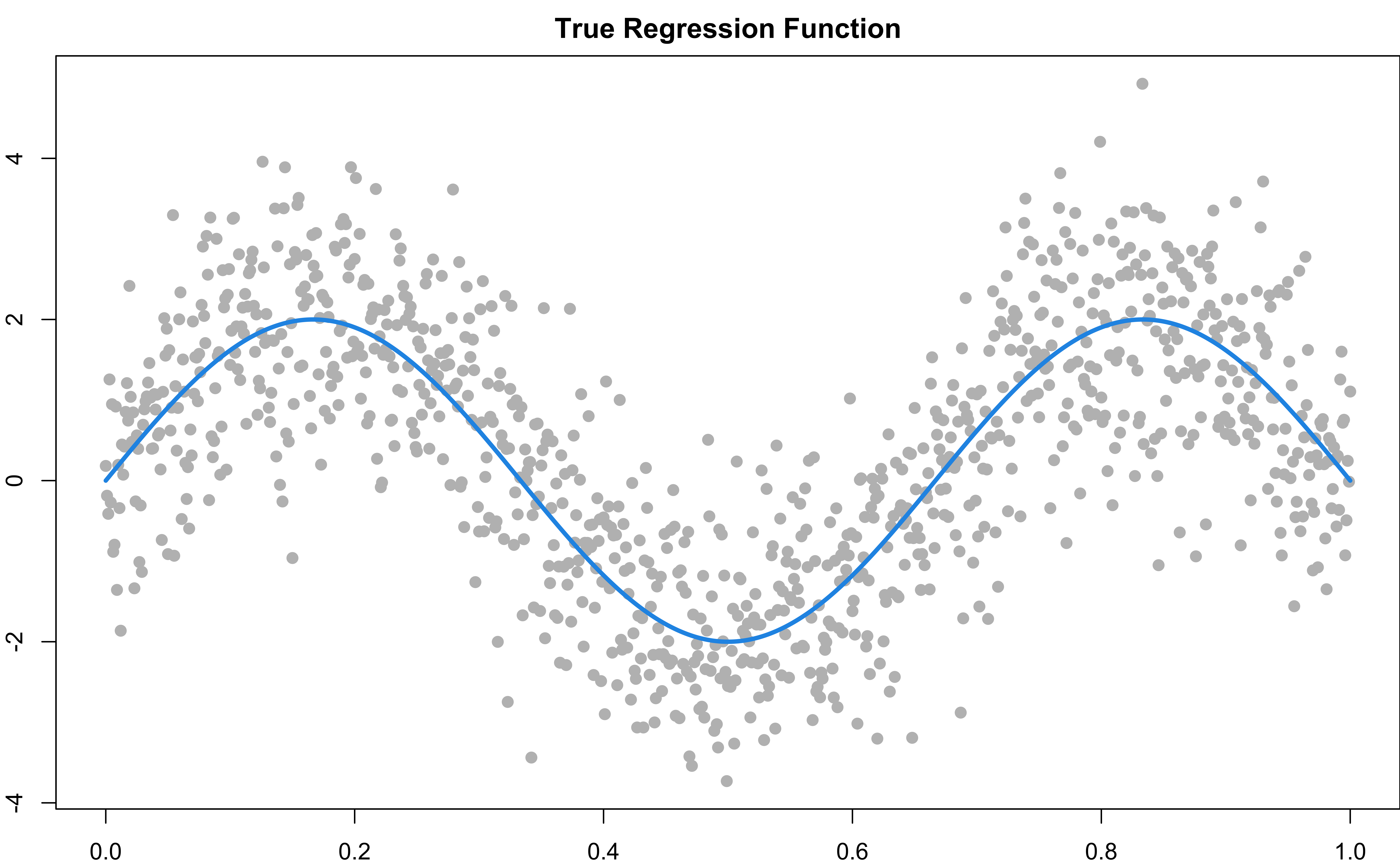
Boosting for Regression
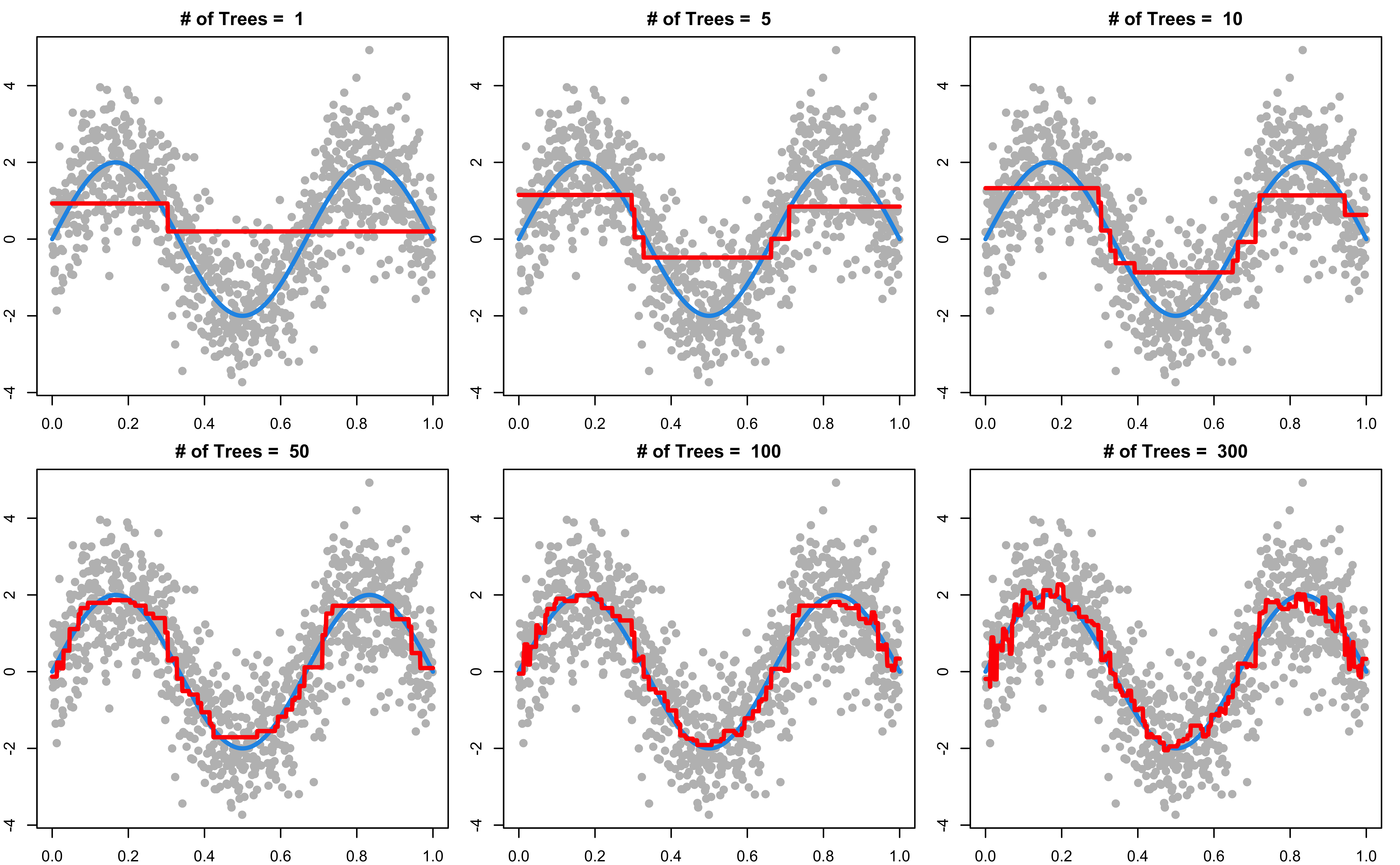
Other Topics
AdaBoost (Adaptive Boosting)
gbm(y ~ ., distribution = "adaboost")-
Gradient Boosting/Extreme Gradient Boosting (XGBoost)
xgboost Bayesian Additive Regression Trees (BART) (ISL Sec. 8.2.4)